Partial Eta Squared for ANOVA from F and Sum of Squares
Description
The formula for $\eta_p^2$ is: $$\frac{SS_{model}} {SS_{model} + SS_{error}}$$
R Function
eta.partial.SS(dfm, dfe, ssm, sse, Fvalue, a)
Arguments
- dfm = degrees of freedom for the model/IV/between
- dfe = degrees of freedom for the error/residual/within
- ssm = sum of squares for the model/IV/between
- sse = sum of squares for the error/residual/within
- Fvalue = F statistic
- a = significance level
Example
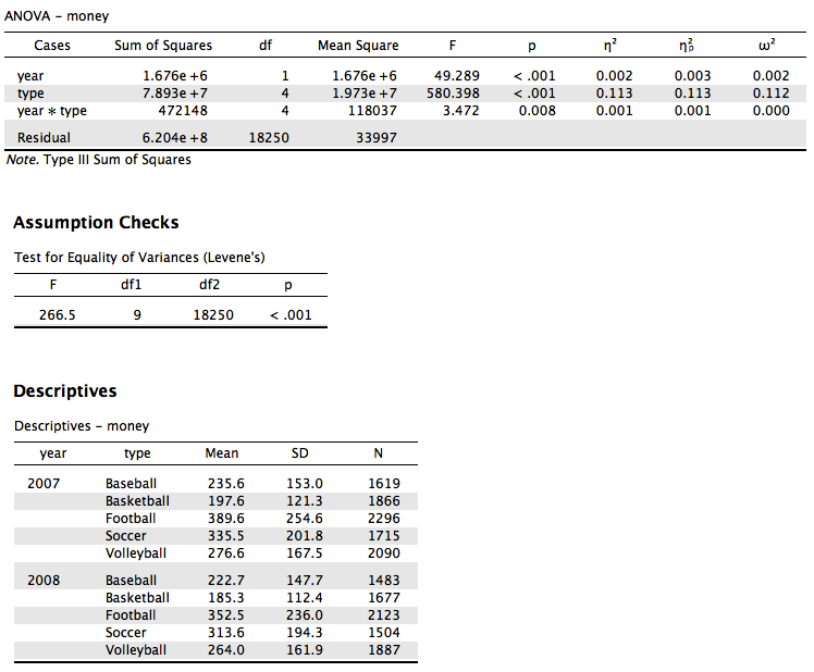
We looked at two year’s worth of athletic spending data (treating each receipt and years as separate between subjects’ events) for four different sports. Are there differences across sports and years in spending? The data are available on GitHub. Example output from JASP, SPSS, and SAS are shown below.
JASP
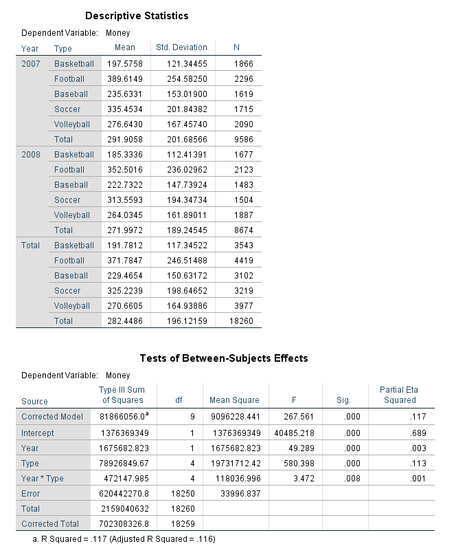
SPSS
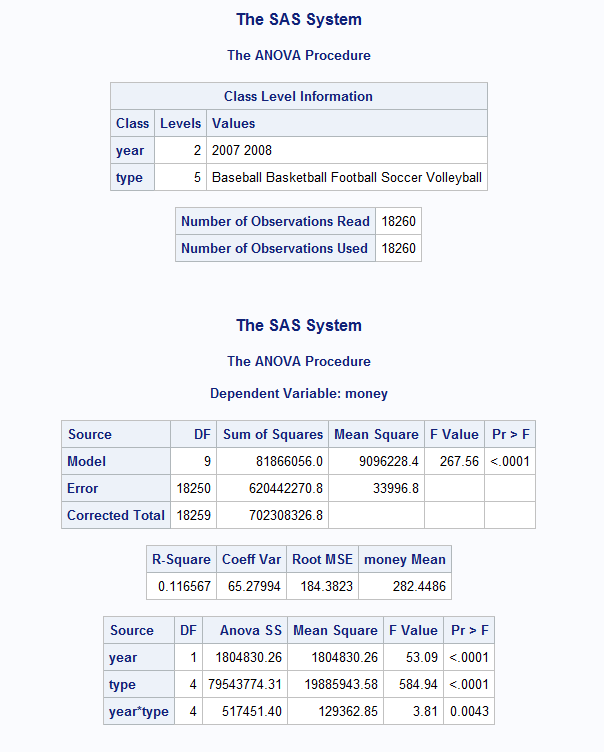
SAS
Function in R:
eta.partial.SS(dfm = 1, dfe = 18250, ssm = 1675682.823, sse = 620442270.8, Fvalue = 49.289, a = .05)
MOTE
Screenshot
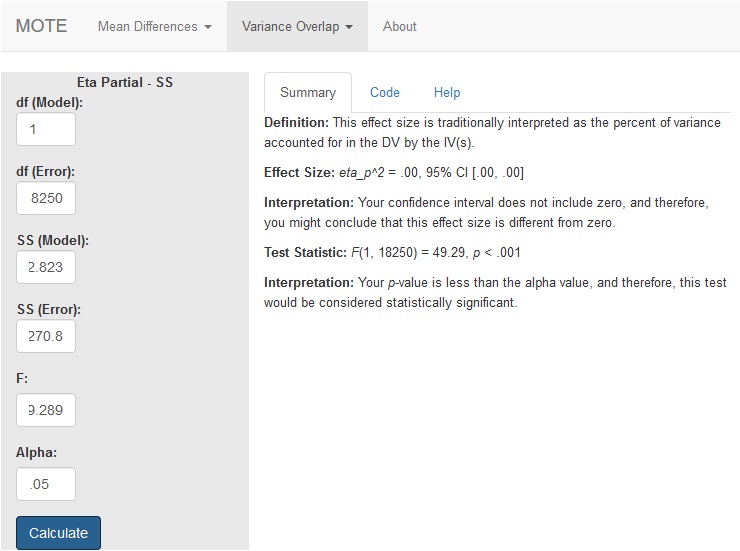
Effect Size:
$\eta_p^2$ = .00, 95% CI [.00, .00]
Interpretation:
Your confidence interval does not include zero, and therefore, you might conclude that this effect size is different from zero.
Summary Statistics:
Not applicable.
Test Statistic:
F(1, 18250) = 49.29, p < .001
Interpretation:
Your p-value is less than the alpha value, and therefore, this test would be considered statistically significant.
