Terms and Concepts

Structural Equation Modeling

• Regression on steroids
• Model many relationships at once, rather than run single regressions
• Model variables that don’t technically exist!

Structural Equation Modeling

• Model theorized causal relationships
  • Even if we did not measure them in a causal way, we can specify direction
• A mostly confirmatory procedure
  • Generally, you have a theory about the relationship before hand
  • Less descriptive/exploratory than traditional hypothesis testing
• Specific error control
  • You can be more specific about the error terms, rather than just one overall residual

Concepts

• Latent variables
  • Represented by circles
  • Abstract phenomena you are trying to model
  • Are not represented by a number in the dataset
  • Linked to the measured variables
  • Represented indirectly by those variables

Concepts

• Manifest or observed variables
  • Represented by squares
  • Measured from participants, business data, or other sources
  • While most measured variables are continuous, you can use categorical and ordered measures as well

Concepts

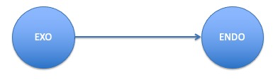
• Exogenous
  • These are synonymous with independent variables
  • They are thought to be the cause of something.
  • You can find these in a model where the arrow is leaving the variable
  • Exogenous (only) variables do not have an error term
  • Changes in these variables are represented by something else you aren’t modeling (like age, gender, etc.)

Concepts

• Endogenous
  • These are synonymous with dependent variables
  • They are caused by the exogenous variables
  • In a model diagram, the arrow will be coming into the variable
  • Endogenous variables have error terms (assigned automatically by the software)

Concepts

• Remember that Y ~ X + $\epsilon$
• Here that is Endogenous ~ Exogenous + Residual
• Sometimes people call residuals: disturbances

Concepts

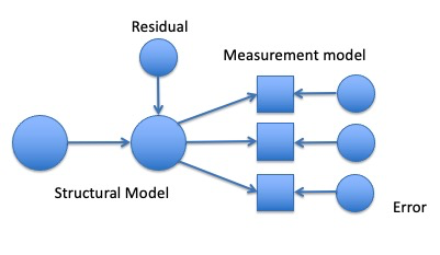
• Measurement model
  • The relationship between an exogenous latent variable and measured variables only.
  • Generally used when describing a confirmatory factor analysis

Concepts

• Full SEM or fully latent SEM
  • A measurement model + causal relationships between latent variables

Concepts

Concepts

• Recursive models – arrows go only in one direction

Concepts

• Nonrecursive models – arrows go backwards to original variables

Interpreting a SEM Diagram

• Recap:
• Circles are latent variables or error terms
  • They do not have numbers in the dataset
• Squares are measured or manifest variables
  • They will have a number in the dataset
• Single headed arrows indicate predicted direction of relationship (–>)
• Double headed arrows indicate variance or covariance (<–>)

Parameters

Unstandardized estimates

• Single arrows are:
  • Between two variables that aren’t latent –> measured: regressions ~
  • Between measured and latents: latent variables =~
  • Indicate the coefficient b - the relationship between these two variables, like regression
• Double arrows are:
  • Covariances ~~: the amount two variables vary together
  • Remember that covariance is not scaled

Parameters

#> lavaan 0.6-19 ended normally after 35 iterations
#> 
#>   Estimator                                         ML
#>   Optimization method                           NLMINB
#>   Number of model parameters                        20
#> 
#>   Number of observations                           301
#> 
#> Model Test User Model:
#>                                                       
#>   Test statistic                               104.570
#>   Degrees of freedom                                25
#>   P-value (Chi-square)                           0.000
#> 
#> Parameter Estimates:
#> 
#>   Standard errors                             Standard
#>   Information                                 Expected
#>   Information saturated (h1) model          Structured
#> 
#> Latent Variables:
#>                    Estimate  Std.Err  z-value  P(>|z|)
#>   visual =~                                           
#>     x1                1.000                           
#>     x2                0.643    0.114    5.650    0.000
#>     x3                0.899    0.135    6.637    0.000
#>   textual =~                                          
#>     x4                1.000                           
#>     x5                1.129    0.066   16.992    0.000
#>     x6                0.926    0.056   16.499    0.000
#>   speed =~                                            
#>     x7                1.000                           
#>     x8                1.178    0.176    6.695    0.000
#>     x9                1.304    0.193    6.774    0.000
#> 
#> Regressions:
#>                    Estimate  Std.Err  z-value  P(>|z|)
#>   visual ~                                            
#>     speed             0.831    0.159    5.215    0.000
#> 
#> Covariances:
#>                    Estimate  Std.Err  z-value  P(>|z|)
#>   textual ~~                                          
#>     speed             0.196    0.048    4.118    0.000
#> 
#> Variances:
#>                    Estimate  Std.Err  z-value  P(>|z|)
#>    .x1                0.694    0.107    6.470    0.000
#>    .x2                1.107    0.102   10.848    0.000
#>    .x3                0.738    0.096    7.696    0.000
#>    .x4                0.381    0.048    7.867    0.000
#>    .x5                0.423    0.058    7.227    0.000
#>    .x6                0.365    0.044    8.368    0.000
#>    .x7                0.869    0.083   10.494    0.000
#>    .x8                0.585    0.070    8.383    0.000
#>    .x9                0.480    0.072    6.685    0.000
#>    .visual            0.447    0.103    4.324    0.000
#>     textual           0.970    0.112    8.664    0.000
#>     speed             0.315    0.078    4.019    0.000

Parameters

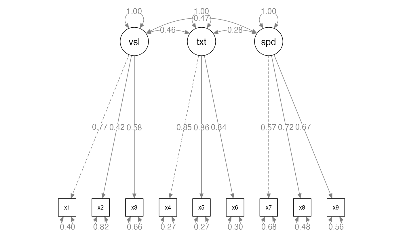
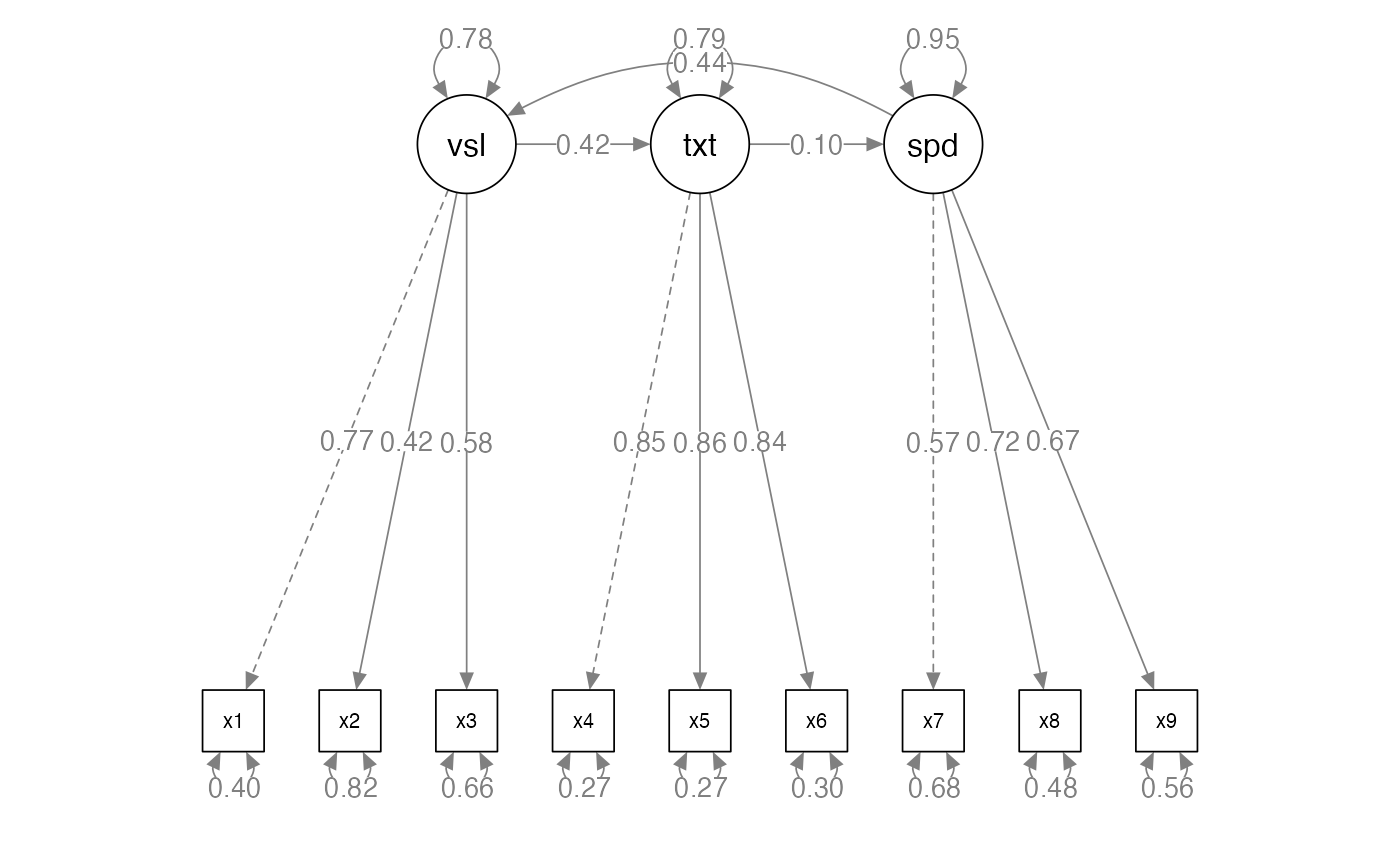
Standardized estimates: note there are several ways to “standardize” the solution, we will cover this more later

• Single arrows are:
  • Regressions ~: the $\beta$ coefficient, z-scored b
  • Latent variables =~: the correlation between a measured and latent variable, usually called loadings like EFA
• Double arrows are:
  • Covariance ~~: the correlation between two variables
• R-Squared: SMCs, Squared Multiple Correlation: variance accounted for in that endogenous variable

Parameters

#> lavaan 0.6-19 ended normally after 35 iterations
#> 
#>   Estimator                                         ML
#>   Optimization method                           NLMINB
#>   Number of model parameters                        20
#> 
#>   Number of observations                           301
#> 
#> Model Test User Model:
#>                                                       
#>   Test statistic                               104.570
#>   Degrees of freedom                                25
#>   P-value (Chi-square)                           0.000
#> 
#> Parameter Estimates:
#> 
#>   Standard errors                             Standard
#>   Information                                 Expected
#>   Information saturated (h1) model          Structured
#> 
#> Latent Variables:
#>                    Estimate  Std.Err  z-value  P(>|z|)   Std.lv  Std.all
#>   visual =~                                                             
#>     x1                1.000                               0.815    0.700
#>     x2                0.643    0.114    5.650    0.000    0.524    0.446
#>     x3                0.899    0.135    6.637    0.000    0.733    0.649
#>   textual =~                                                            
#>     x4                1.000                               0.985    0.847
#>     x5                1.129    0.066   16.992    0.000    1.112    0.863
#>     x6                0.926    0.056   16.499    0.000    0.912    0.834
#>   speed =~                                                              
#>     x7                1.000                               0.561    0.516
#>     x8                1.178    0.176    6.695    0.000    0.661    0.654
#>     x9                1.304    0.193    6.774    0.000    0.731    0.726
#> 
#> Regressions:
#>                    Estimate  Std.Err  z-value  P(>|z|)   Std.lv  Std.all
#>   visual ~                                                              
#>     speed             0.831    0.159    5.215    0.000    0.572    0.572
#> 
#> Covariances:
#>                    Estimate  Std.Err  z-value  P(>|z|)   Std.lv  Std.all
#>   textual ~~                                                            
#>     speed             0.196    0.048    4.118    0.000    0.354    0.354
#> 
#> Variances:
#>                    Estimate  Std.Err  z-value  P(>|z|)   Std.lv  Std.all
#>    .x1                0.694    0.107    6.470    0.000    0.694    0.511
#>    .x2                1.107    0.102   10.848    0.000    1.107    0.801
#>    .x3                0.738    0.096    7.696    0.000    0.738    0.579
#>    .x4                0.381    0.048    7.867    0.000    0.381    0.282
#>    .x5                0.423    0.058    7.227    0.000    0.423    0.255
#>    .x6                0.365    0.044    8.368    0.000    0.365    0.305
#>    .x7                0.869    0.083   10.494    0.000    0.869    0.734
#>    .x8                0.585    0.070    8.383    0.000    0.585    0.573
#>    .x9                0.480    0.072    6.685    0.000    0.480    0.473
#>    .visual            0.447    0.103    4.324    0.000    0.673    0.673
#>     textual           0.970    0.112    8.664    0.000    1.000    1.000
#>     speed             0.315    0.078    4.019    0.000    1.000    1.000
#> 
#> R-Square:
#>                    Estimate
#>     x1                0.489
#>     x2                0.199
#>     x3                0.421
#>     x4                0.718
#>     x5                0.745
#>     x6                0.695
#>     x7                0.266
#>     x8                0.427
#>     x9                0.527
#>     visual            0.327

Types of Research Questions

• Adequacy of the model
  • Model fit, $\chi^2$, and fit indices
  • No errors or Heywood cases
  • Low residuals, modification indices
• Testing Theory
  • Path significance: note large sample sizes, instead path size
  • Are there better competing models?
  • Modification indices

Types of Research Questions

• Amount of variance (effect size): SMCS $R^2$
• Parameter Estimates: direction and strength
• Group differences:
  • Multi-group models, multiple indicators models (MIMIC)
• Longitudinal differences with Latent Growth Curves
• Multilevel modeling on repeated measures datasets

Practical Issues

• Sample size: for parameter estimates to be accurate, you should have large samples
• How many? Hard to say, but often hundreds are necessary
• http://web.pdx.edu/~newsomj/semclass/ho_sample%20size.pdf
• https://www.ncbi.nlm.nih.gov/pmc/articles/PMC4334479/

Practical Issues

• Sample Size: The N:q rule
  • Number of people, N
  • q number of estimated parameters
  • You want the N:q ratio to be 20:1 or greater in a perfect world, 10:1 if you can manage it.

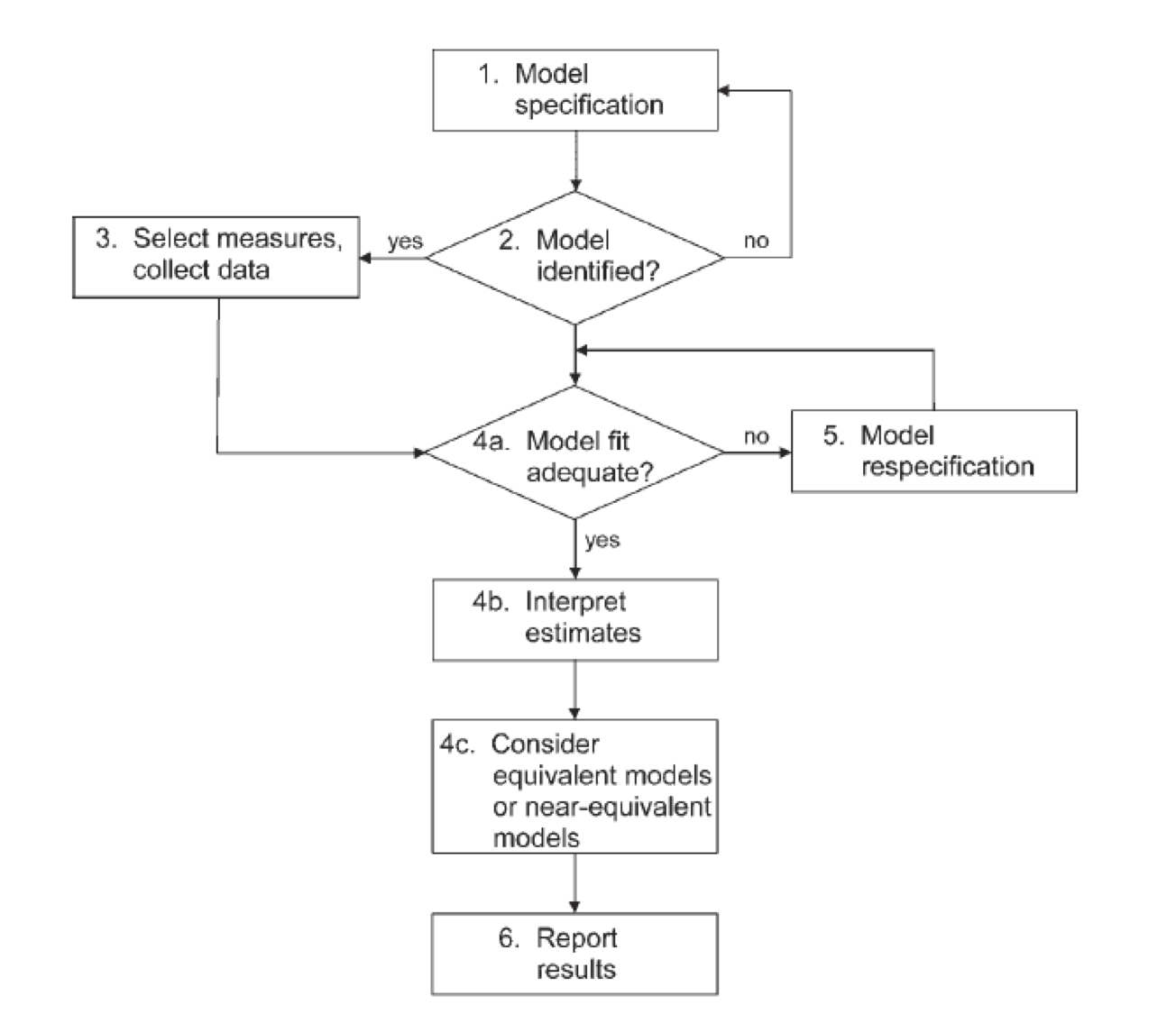
Hypothesis Testing

• Theory + Model Building
• Get the data
• Build the model
• Run the model
• Examine model fit with fit statistics
• Update, replicate

Hypothesis Testing

• Examining model fit is based on residuals
  • Residuals are the error terms
  • Y ~ X + $\epsilon$
  • Want the residuals to be as small as possible
  • Those residuals are estimated from model (i.e., they are circles)
  • Smaller error implies that the model and data match - a more accurate representation of the relationships you are trying to model

Approaches to Modeling

• Strictly confirmatory
  • You have a theorized model and you accept or reject it only.
• Alternative models
  • Comparison between many different models of the construct
  • These models are common in scale development, comparing the number of expected factors
• Model generating
  • The original model doesn’t work, so you improve it for further testing
  • Sometimes called E-SEM

Approaches to Modeling

Specification

• Specification is:
  • Generating the model hypothesis
  • Drawing out how you think the variables are related
  • Defining the model code
• Errors:
  • LOVE: left out variable error
  • Omitted predictors that are important but left out
  • Practically: you diagrammed something wrong, typed the code incorrectly, etc.

Identification

• To be able to understand identification, you have to understand that SEM is an analysis of covariances
• You are trying to explain as much of the variance between variables with your model
• You can also estimate a mean structure
  • Often used in multigroup analysis

Identification

• Models that are identified have a unique answer
  • 2x = 4 has one answer
  • 2x + y = 10 has many answers
• Models that are identified have one probable answer for all the parameters you are estimating

Identification

• Identification is tied to:
  • Parameters to be estimated
  • Degrees of Freedom
• Most software programs help you out but always look for warnings

Identification

• Free parameter – will be estimated from the data
• Fixed parameter – will be set to a specific value
  • Sometimes set to 1 as an indicator or marker variable
    
  • Sometimes practically set when model issues arise
• Constrained parameter – estimated from the data with some specific rule
  • Setting a value equal to another parameter
  • Also known as an equality constraint
  • Cross group equality constraints – mostly used in multigroup models, forces the same paths to be equal (but estimated) for each group

Identifying What’s What

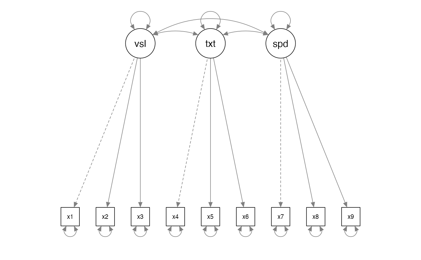
• 3 variances on latent variables
• 3 covariances between latent variables
• 6 latent variable loadings
• 9 error variances

Identifying What’s What

• Degrees of Freedom
  • DF is not related to sample size
• Calculate possible parameters: $\frac{p \times (p+1)}{2}$
  • P is the number of measured variables
  • $\frac{9 \times (9+1)}{2}$ = 45
• Subtract the number of estimated parameters
  • 45 - 21 = 24

Identifying What’s What

• Did we get it right?

#> lavaan 0.6-19 ended normally after 35 iterations
#> 
#>   Estimator                                         ML
#>   Optimization method                           NLMINB
#>   Number of model parameters                        21
#> 
#>   Number of observations                           301
#> 
#> Model Test User Model:
#>                                                       
#>   Test statistic                                85.306
#>   Degrees of freedom                                24
#>   P-value (Chi-square)                           0.000
#> 
#> Parameter Estimates:
#> 
#>   Standard errors                             Standard
#>   Information                                 Expected
#>   Information saturated (h1) model          Structured
#> 
#> Latent Variables:
#>                    Estimate  Std.Err  z-value  P(>|z|)
#>   visual =~                                           
#>     x1                1.000                           
#>     x2                0.554    0.100    5.554    0.000
#>     x3                0.729    0.109    6.685    0.000
#>   textual =~                                          
#>     x4                1.000                           
#>     x5                1.113    0.065   17.014    0.000
#>     x6                0.926    0.055   16.703    0.000
#>   speed =~                                            
#>     x7                1.000                           
#>     x8                1.180    0.165    7.152    0.000
#>     x9                1.082    0.151    7.155    0.000
#> 
#> Covariances:
#>                    Estimate  Std.Err  z-value  P(>|z|)
#>   visual ~~                                           
#>     textual           0.408    0.074    5.552    0.000
#>     speed             0.262    0.056    4.660    0.000
#>   textual ~~                                          
#>     speed             0.173    0.049    3.518    0.000
#> 
#> Variances:
#>                    Estimate  Std.Err  z-value  P(>|z|)
#>    .x1                0.549    0.114    4.833    0.000
#>    .x2                1.134    0.102   11.146    0.000
#>    .x3                0.844    0.091    9.317    0.000
#>    .x4                0.371    0.048    7.779    0.000
#>    .x5                0.446    0.058    7.642    0.000
#>    .x6                0.356    0.043    8.277    0.000
#>    .x7                0.799    0.081    9.823    0.000
#>    .x8                0.488    0.074    6.573    0.000
#>    .x9                0.566    0.071    8.003    0.000
#>     visual            0.809    0.145    5.564    0.000
#>     textual           0.979    0.112    8.737    0.000
#>     speed             0.384    0.086    4.451    0.000

Identification

• Just identified models mean the df = 0
  • Generally, not a good sign
  • Cross panel lagged models are set up this way on purpose
• Over identified models mean df > 0
  • You want this!
• Under identified models mean the df < 0
  • You can’t run this!

Identification

• Empirical under identification
  • When two observed variables are highly correlated, which effectively reduces the number of parameters you can estimate
• Even if you have an over identified model, you can have under identified sections

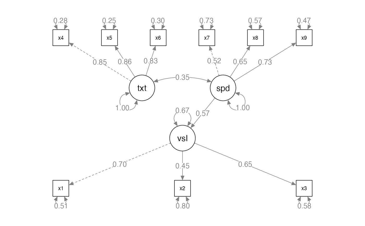
Identification

• How do I create identified models?
  • Scaling/reference/marker variables: a parameter you set to 1
  • Helps increase df by eliminating a free parameter
  • Gives the model a scale
  • Can be done in a couple of ways, generally on the measurement model
  • Pay attention to the number of variables attached to a latent variable in a measurement model

Identification

• Does the marker variable matter?
  • No, it should not change the model if you change which variable you set it to
  • If it does, something is likely weird with your model
  • The reference variable will not have an estimated unstandardized parameter
  • You will get a standardized parameter, so you can check if the variable is loading like what you think it should
  • If you need a p-value for that parameter, you can run the model twice

Identification

#> lavaan 0.6-19 ended normally after 35 iterations
#> 
#>   Estimator                                         ML
#>   Optimization method                           NLMINB
#>   Number of model parameters                        21
#> 
#>   Number of observations                           301
#> 
#> Model Test User Model:
#>                                                       
#>   Test statistic                                85.306
#>   Degrees of freedom                                24
#>   P-value (Chi-square)                           0.000
#> 
#> Parameter Estimates:
#> 
#>   Standard errors                             Standard
#>   Information                                 Expected
#>   Information saturated (h1) model          Structured
#> 
#> Latent Variables:
#>                    Estimate  Std.Err  z-value  P(>|z|)   Std.lv  Std.all
#>   visual =~                                                             
#>     x1                1.000                               0.900    0.772
#>     x2                0.554    0.100    5.554    0.000    0.498    0.424
#>     x3                0.729    0.109    6.685    0.000    0.656    0.581
#>   textual =~                                                            
#>     x4                1.000                               0.990    0.852
#>     x5                1.113    0.065   17.014    0.000    1.102    0.855
#>     x6                0.926    0.055   16.703    0.000    0.917    0.838
#>   speed =~                                                              
#>     x7                1.000                               0.619    0.570
#>     x8                1.180    0.165    7.152    0.000    0.731    0.723
#>     x9                1.082    0.151    7.155    0.000    0.670    0.665
#> 
#> Covariances:
#>                    Estimate  Std.Err  z-value  P(>|z|)   Std.lv  Std.all
#>   visual ~~                                                             
#>     textual           0.408    0.074    5.552    0.000    0.459    0.459
#>     speed             0.262    0.056    4.660    0.000    0.471    0.471
#>   textual ~~                                                            
#>     speed             0.173    0.049    3.518    0.000    0.283    0.283
#> 
#> Variances:
#>                    Estimate  Std.Err  z-value  P(>|z|)   Std.lv  Std.all
#>    .x1                0.549    0.114    4.833    0.000    0.549    0.404
#>    .x2                1.134    0.102   11.146    0.000    1.134    0.821
#>    .x3                0.844    0.091    9.317    0.000    0.844    0.662
#>    .x4                0.371    0.048    7.779    0.000    0.371    0.275
#>    .x5                0.446    0.058    7.642    0.000    0.446    0.269
#>    .x6                0.356    0.043    8.277    0.000    0.356    0.298
#>    .x7                0.799    0.081    9.823    0.000    0.799    0.676
#>    .x8                0.488    0.074    6.573    0.000    0.488    0.477
#>    .x9                0.566    0.071    8.003    0.000    0.566    0.558
#>     visual            0.809    0.145    5.564    0.000    1.000    1.000
#>     textual           0.979    0.112    8.737    0.000    1.000    1.000
#>     speed             0.384    0.086    4.451    0.000    1.000    1.000

Identification

• If you have a complex model:
  • Start small – work with the measurement model components first, since they have simple identification rules
  • Then work up to adding variables to see where the problem occurs
  • lavaan gives you somewhat good warnings
  • Page 130 Kline has a great set of references for identification

Positive Definite Matrices

• Dreaded: hessian matrix not definite
• What that indicates is the following:
  • Matrix is singular
  • Eigenvalues are negative
  • Determinants are zero or negative
  • Correlations are out of bounds

Positive Definite Matrices

• Simply put: each column has to indicate something unique
  • Therefore, if you have two columns that are perfectly correlated OR are linear transformations of each other, you will have a singular matrix
• Negative eigenvalues – remember that eigenvalues are combinations of variance
  • And variance is positive (it’s squared in the formula!)
• Determinants are the products of eigenvalues
  • Again, they cannot be negative
  • A zero determinant indicates a singular matrix
• Out of bounds – basically that means that the data has correlations over 1 or negative variances (Heywood case)

Summary

In this lecture you’ve learned:

• Basic terminology
• Beginning to map pictures to code definition (~) to output
• Beginning steps to specifying and creating identified models
• Degrees of freedom
• Errors you may encounter