Latent Growth Models
lecture_lgm.RmdLatent Growth Modeling
- Measuring change over repeated time measurements
- Gives you more information than a traditional repeated measures ANOVA or regression line by itself.
- Advantages:
- Estimate means and covariances separately
- Estimating observed values and unobserved values separately
Assumptions
- Continuous measurement of the DVs
- This assumption is true for many structural models though!
- Time spacing is the same across people
- NOT across measurements, but people need to be spaced the same
- At least three time points per person (otherwise, you are doing a dependent t-test)
- Large samples!
Before you start
- You have to know the expected type of change before you start
- Generally it’s linear, however, you can do curvilinear or power functions
Example model
- We will set the regression loading values to specific numbers to be able to estimate intercept and slope.
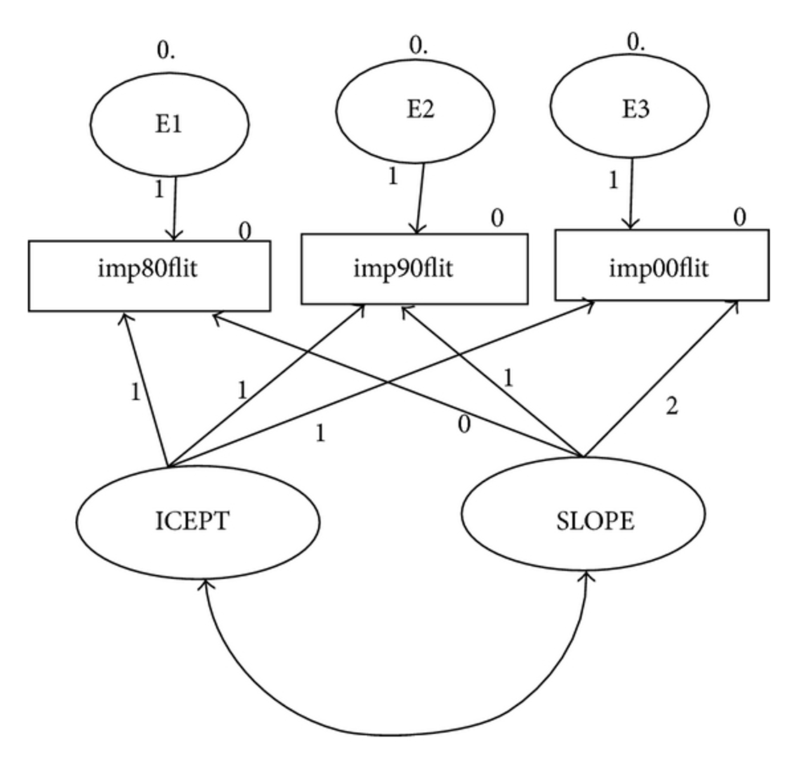
Understand the idea
- Intercept
- You set these values to 1 indicating that you do NOT want to estimate them
- Basically, that gives you a starting value for the first time point, which is the average point where people start (y-intercept)
Understand the idea
- Slope – represents the change over time
- You can set these values to anything you want
- Usually the first time is indicated by a 0
- There’s no slope for time 1, just an intercept
- Then the paths are set based on the time differences between them
Understand the idea
- Setting the parameters this way:
- Helps with identification
- Is theoretical to match the concept of slope and intercept estimation
- Allows you to not have to set the variances, so you can look at them
Questions
- What is the average change for each person?
- Where do they start?
- How does it change over time?
- What is the form of the change?
Questions
- Is the average slope and intercept a good fit for all participants?
- Or should we include a variance term to account for the differences between people?
- Models are called random effects if you add the random variances (similar to multilevel models)
- If we have a random effects model – is there another variable that explains those random effects?
Understanding the Output
- Intercept mean: the average starting point for time 1
- Slope mean: the average increment across time points
Understanding the Output
- Intercept variance: the spread around the average start point
- Large scores indicate a lot of spread – meaning people start in a lot of different places
- Small scores indicate a small spread – everyone starts about the same place
Understanding the Output
- Slope variance – the range of increments across time points
- Small variances mean that everyone is going up/down about the same amount
- Large variances mean that people scores are going up/down differently (almost like an interaction)
Understanding the Output
- Factor covariance – examines the relationship between intercept and slope
- Positive covariance - positive slope
- People who start with higher intercepts have higher positive slopes
- Positive covariance - negative slope
- People who start higher go down faster (larger negative slopes)
- Negative covariance - positive slope
- People who start with higher intercepts go up slower (smaller slopes)
- Negative covariance - negative slope
- People who start with higher intercepts go down slower
New Functions
-
growth(): This function helps with the set up for a LCM, fixes the parameters correctly for you. - We will use the data as covariances and means, but you can import
the data just like
cfa()
How to Test
- This procedure is very similar to multigroup model testing, only in reverse.
- We are going to start with the most constrained model and slowly let parameters free to see which is the best.
- We would prefer the unconstrained model be the best:
- The slope and intercept are useful
- But the variances to be low indicating everyone has the same pattern of slope and intercept
Intercept Only Model
- Use only the intercept (mean of the data) to estimate
- You want this model to be bad, otherwise you are saying that one average score is the best for all the time points
- Intercept variance is constrained to 0, so you only get a mean.
- Residuals are forced to be the same for each time point, so the variance is the same across all time points
crime.model1 <- '
# intercept
i =~ 1*Time1 + 1*Time2 + 1*Time3 + 1*Time4
i~~0*i
# residual variances
Time1~~r*Time1
Time2~~r*Time2
Time3~~r*Time3
Time4~~r*Time4
'
Intercept Only Model
crime.fit1 <- growth(crime.model1,
                    sample.cov=crime.cov,
                    sample.mean=crime.mean,
                    sample.nobs=952)
summary(crime.fit1,
        standardized = TRUE,
        fit.measures = TRUE,
        rsquare = TRUE)
#> lavaan 0.6-19 ended normally after 19 iterations
#>
#>   Estimator                                         ML
#>   Optimization method                           NLMINB
#>   Number of model parameters                         5
#>   Number of equality constraints                     3
#>
#>   Number of observations                           952
#>
#> Model Test User Model:
#>
#>   Test statistic                              3461.981
#>   Degrees of freedom                                12
#>   P-value (Chi-square)                           0.000
#>
#> Model Test Baseline Model:
#>
#>   Test statistic                              3358.206
#>   Degrees of freedom                                 6
#>   P-value                                        0.000
#>
#> User Model versus Baseline Model:
#>
#>   Comparative Fit Index (CFI)                    0.000
#>   Tucker-Lewis Index (TLI)                       0.485
#>
#> Loglikelihood and Information Criteria:
#>
#>   Loglikelihood user model (H0)              -4540.205
#>   Loglikelihood unrestricted model (H1)      -2809.215
#>
#>   Akaike (AIC)                                9084.410
#>   Bayesian (BIC)                              9094.127
#>   Sample-size adjusted Bayesian (SABIC)       9087.775
#>
#> Root Mean Square Error of Approximation:
#>
#>   RMSEA                                          0.550
#>   90 Percent confidence interval - lower         0.534
#>   90 Percent confidence interval - upper         0.565
#>   P-value H_0: RMSEA <= 0.050                    0.000
#>   P-value H_0: RMSEA >= 0.080                    1.000
#>
#> Standardized Root Mean Square Residual:
#>
#>   SRMR                                           0.523
#>
#> Parameter Estimates:
#>
#>   Standard errors                             Standard
#>   Information                                 Expected
#>   Information saturated (h1) model          Structured
#>
#> Latent Variables:
#>                    Estimate  Std.Err  z-value  P(>|z|)   Std.lv  Std.all
#>   i =~
#>     Time1             1.000                               0.000    0.000
#>     Time2             1.000                               0.000    0.000
#>     Time3             1.000                               0.000    0.000
#>     Time4             1.000                               0.000    0.000
#>
#> Intercepts:
#>                    Estimate  Std.Err  z-value  P(>|z|)   Std.lv  Std.all
#>     i                 5.352    0.013  414.325    0.000      Inf      Inf
#>
#> Variances:
#>                    Estimate  Std.Err  z-value  P(>|z|)   Std.lv  Std.all
#>     i                 0.000                                 NaN      NaN
#>    .Time1      (r)    0.636    0.015   43.635    0.000    0.636    1.000
#>    .Time2      (r)    0.636    0.015   43.635    0.000    0.636    1.000
#>    .Time3      (r)    0.636    0.015   43.635    0.000    0.636    1.000
#>    .Time4      (r)    0.636    0.015   43.635    0.000    0.636    1.000
#>
#> R-Square:
#>                    Estimate
#>     Time1             0.000
#>     Time2             0.000
#>     Time3             0.000
#>     Time4             0.000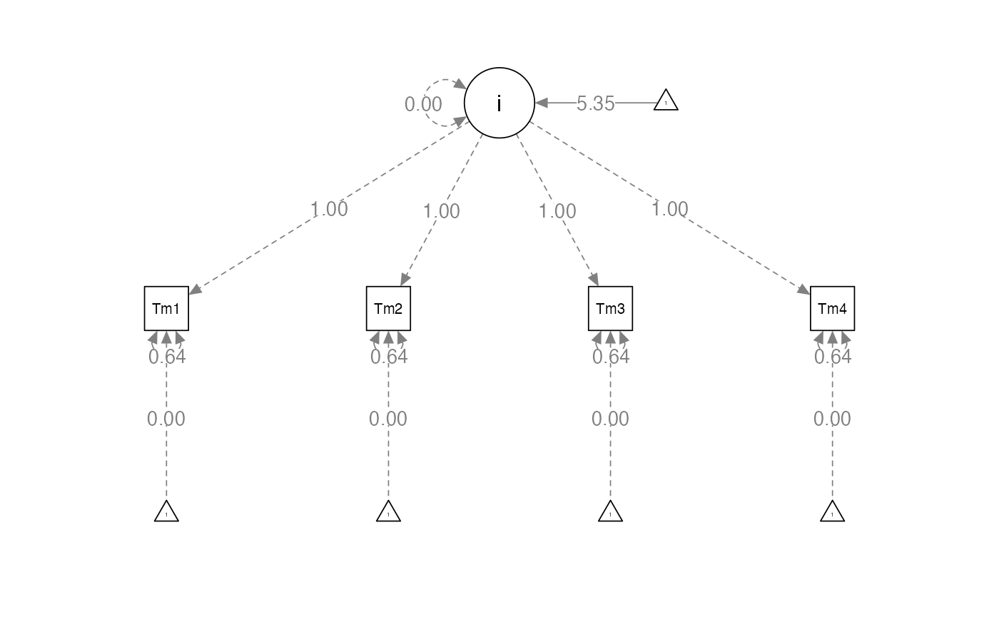
Comparison Table Fit Indices
library(knitr)
fit.table <- matrix(NA, nrow = 5, ncol = 6)
colnames(fit.table) <- c("Model", "X2", "df", "RMSEA", "SRMR", "CFI")
fit.table[1, ] <- c("Intercept Only", round(fitmeasures(crime.fit1, c("chisq", "df", "rmsea", "srmr", "cfi")),3))
kable(fit.table)| Model | X2 | df | RMSEA | SRMR | CFI |
|---|---|---|---|---|---|
| Intercept Only | 3461.981 | 12 | 0.55 | 0.523 | 0 |
| NA | NA | NA | NA | NA | NA |
| NA | NA | NA | NA | NA | NA |
| NA | NA | NA | NA | NA | NA |
| NA | NA | NA | NA | NA | NA |
Comparison Table Parameters
#save the parameter estimates
crime.fit1.par <- parameterestimates(crime.fit1)

#make table
par.table <- matrix(NA, nrow = 5, ncol = 7)
colnames(par.table) <- c("Model", "Intercept Mean", "Intercept Variance", "Residual Variance", "Slope Mean", "Slope Variance", "Covariance")

#put data in table
par.table[1, ] <- c("Intercept Only",
                    round(crime.fit1.par$est[crime.fit1.par$lhs == "i" & crime.fit1.par$op == "~1"], 3),
                    "X",
                    round(crime.fit1.par$est[crime.fit1.par$lhs == "Time1" & crime.fit1.par$op == "~~"], 3),
                    "X",
                    "X",
                    "X")
kable(par.table)| Model | Intercept Mean | Intercept Variance | Residual Variance | Slope Mean | Slope Variance | Covariance |
|---|---|---|---|---|---|---|
| Intercept Only | 5.352 | X | 0.636 | X | X | X |
| NA | NA | NA | NA | NA | NA | NA |
| NA | NA | NA | NA | NA | NA | NA |
| NA | NA | NA | NA | NA | NA | NA |
| NA | NA | NA | NA | NA | NA | NA |
Random Intercept Only Model
- We allow the intercept variance to be > 0
- People can start at different places
- Residual variances are still the same
- Still no slope
crime.model2 <- '
# intercept
i =~ 1*Time1 + 1*Time2 + 1*Time3 + 1*Time4
# residual variances
Time1~~r*Time1
Time2~~r*Time2
Time3~~r*Time3
Time4~~r*Time4
'
Random Intercept Only Model
crime.fit2 <- growth(crime.model2,
                    sample.cov=crime.cov,
                    sample.mean=crime.mean,
                    sample.nobs=952)
summary(crime.fit2,
        standardized = TRUE,
        fit.measures = TRUE,
        rsquare = TRUE)
#> lavaan 0.6-19 ended normally after 19 iterations
#>
#>   Estimator                                         ML
#>   Optimization method                           NLMINB
#>   Number of model parameters                         6
#>   Number of equality constraints                     3
#>
#>   Number of observations                           952
#>
#> Model Test User Model:
#>
#>   Test statistic                               555.313
#>   Degrees of freedom                                11
#>   P-value (Chi-square)                           0.000
#>
#> Model Test Baseline Model:
#>
#>   Test statistic                              3358.206
#>   Degrees of freedom                                 6
#>   P-value                                        0.000
#>
#> User Model versus Baseline Model:
#>
#>   Comparative Fit Index (CFI)                    0.838
#>   Tucker-Lewis Index (TLI)                       0.911
#>
#> Loglikelihood and Information Criteria:
#>
#>   Loglikelihood user model (H0)              -3086.871
#>   Loglikelihood unrestricted model (H1)      -2809.215
#>
#>   Akaike (AIC)                                6179.742
#>   Bayesian (BIC)                              6194.318
#>   Sample-size adjusted Bayesian (SABIC)       6184.790
#>
#> Root Mean Square Error of Approximation:
#>
#>   RMSEA                                          0.228
#>   90 Percent confidence interval - lower         0.212
#>   90 Percent confidence interval - upper         0.244
#>   P-value H_0: RMSEA <= 0.050                    0.000
#>   P-value H_0: RMSEA >= 0.080                    1.000
#>
#> Standardized Root Mean Square Residual:
#>
#>   SRMR                                           0.092
#>
#> Parameter Estimates:
#>
#>   Standard errors                             Standard
#>   Information                                 Expected
#>   Information saturated (h1) model          Structured
#>
#> Latent Variables:
#>                    Estimate  Std.Err  z-value  P(>|z|)   Std.lv  Std.all
#>   i =~
#>     Time1             1.000                               0.693    0.870
#>     Time2             1.000                               0.693    0.870
#>     Time3             1.000                               0.693    0.870
#>     Time4             1.000                               0.693    0.870
#>
#> Intercepts:
#>                    Estimate  Std.Err  z-value  P(>|z|)   Std.lv  Std.all
#>     i                 5.352    0.023  229.140    0.000    7.720    7.720
#>
#> Variances:
#>                    Estimate  Std.Err  z-value  P(>|z|)   Std.lv  Std.all
#>    .Time1      (r)    0.155    0.004   37.789    0.000    0.155    0.244
#>    .Time2      (r)    0.155    0.004   37.789    0.000    0.155    0.244
#>    .Time3      (r)    0.155    0.004   37.789    0.000    0.155    0.244
#>    .Time4      (r)    0.155    0.004   37.789    0.000    0.155    0.244
#>     i                 0.481    0.024   20.174    0.000    1.000    1.000
#>
#> R-Square:
#>                    Estimate
#>     Time1             0.756
#>     Time2             0.756
#>     Time3             0.756
#>     Time4             0.756
Comparison Table Fit Indices
- This model is much better than model 1
- Implies that people all start in different places
fit.table[2, ] <- c("Random Intercept", round(fitmeasures(crime.fit2, c("chisq", "df", "rmsea", "srmr", "cfi")),3))
kable(fit.table)| Model | X2 | df | RMSEA | SRMR | CFI |
|---|---|---|---|---|---|
| Intercept Only | 3461.981 | 12 | 0.55 | 0.523 | 0 |
| Random Intercept | 555.313 | 11 | 0.228 | 0.092 | 0.838 |
| NA | NA | NA | NA | NA | NA |
| NA | NA | NA | NA | NA | NA |
| NA | NA | NA | NA | NA | NA |
Comparison Table Parameters
#save the parameter estimates
crime.fit2.par <- parameterestimates(crime.fit2)

#put data in table
par.table[2, ] <- c("Random Intercept",
                    round(crime.fit2.par$est[crime.fit2.par$lhs == "i" & crime.fit2.par$op == "~1"], 3),
                    round(crime.fit2.par$est[crime.fit2.par$lhs == "i" & crime.fit2.par$op == "~~"], 3),
                    round(crime.fit2.par$est[crime.fit2.par$lhs == "Time1" & crime.fit2.par$op == "~~"], 3),
                    "X",
                    "X",
                    "X")
kable(par.table)| Model | Intercept Mean | Intercept Variance | Residual Variance | Slope Mean | Slope Variance | Covariance |
|---|---|---|---|---|---|---|
| Intercept Only | 5.352 | X | 0.636 | X | X | X |
| Random Intercept | 5.352 | 0.481 | 0.155 | X | X | X |
| NA | NA | NA | NA | NA | NA | NA |
| NA | NA | NA | NA | NA | NA | NA |
| NA | NA | NA | NA | NA | NA | NA |
Random Slope + Intercepts
- Add in the random slope
-
s~0*1(makes the average slope 0) -
s~~0*i(uncorrelated slope/intercept)
-
- Leave the intercept and its variance in the model
- Keep the residuals constrained to be the same
crime.model3 <- '
# intercept
i =~ 1*Time1 + 1*Time2 + 1*Time3 + 1*Time4
# slope
s =~ 0*Time1 + 1*Time2 + 2*Time3 + 3*Time4
s~0*1
s~~0*i
# residual variances
Time1~~r*Time1
Time2~~r*Time2
Time3~~r*Time3
Time4~~r*Time4
'
Random Slope + Intercepts
crime.fit3 <- growth(crime.model3,
                    sample.cov=crime.cov,
                    sample.mean=crime.mean,
                    sample.nobs=952)
summary(crime.fit3,
        standardized = TRUE,
        fit.measures = TRUE,
        rsquare = TRUE)
#> lavaan 0.6-19 ended normally after 38 iterations
#>
#>   Estimator                                         ML
#>   Optimization method                           NLMINB
#>   Number of model parameters                         7
#>   Number of equality constraints                     3
#>
#>   Number of observations                           952
#>
#> Model Test User Model:
#>
#>   Test statistic                               339.586
#>   Degrees of freedom                                10
#>   P-value (Chi-square)                           0.000
#>
#> Model Test Baseline Model:
#>
#>   Test statistic                              3358.206
#>   Degrees of freedom                                 6
#>   P-value                                        0.000
#>
#> User Model versus Baseline Model:
#>
#>   Comparative Fit Index (CFI)                    0.902
#>   Tucker-Lewis Index (TLI)                       0.941
#>
#> Loglikelihood and Information Criteria:
#>
#>   Loglikelihood user model (H0)              -2979.008
#>   Loglikelihood unrestricted model (H1)      -2809.215
#>
#>   Akaike (AIC)                                5966.015
#>   Bayesian (BIC)                              5985.450
#>   Sample-size adjusted Bayesian (SABIC)       5972.746
#>
#> Root Mean Square Error of Approximation:
#>
#>   RMSEA                                          0.186
#>   90 Percent confidence interval - lower         0.169
#>   90 Percent confidence interval - upper         0.203
#>   P-value H_0: RMSEA <= 0.050                    0.000
#>   P-value H_0: RMSEA >= 0.080                    1.000
#>
#> Standardized Root Mean Square Residual:
#>
#>   SRMR                                           0.149
#>
#> Parameter Estimates:
#>
#>   Standard errors                             Standard
#>   Information                                 Expected
#>   Information saturated (h1) model          Structured
#>
#> Latent Variables:
#>                    Estimate  Std.Err  z-value  P(>|z|)   Std.lv  Std.all
#>   i =~
#>     Time1             1.000                               0.696    0.903
#>     Time2             1.000                               0.696    0.884
#>     Time3             1.000                               0.696    0.835
#>     Time4             1.000                               0.696    0.768
#>   s =~
#>     Time1             0.000                               0.000    0.000
#>     Time2             1.000                               0.158    0.201
#>     Time3             2.000                               0.317    0.380
#>     Time4             3.000                               0.475    0.525
#>
#> Covariances:
#>                    Estimate  Std.Err  z-value  P(>|z|)   Std.lv  Std.all
#>   i ~~
#>     s                 0.000                               0.000    0.000
#>
#> Intercepts:
#>                    Estimate  Std.Err  z-value  P(>|z|)   Std.lv  Std.all
#>     s                 0.000                               0.000    0.000
#>     i                 5.262    0.024  221.401    0.000    7.565    7.565
#>
#> Variances:
#>                    Estimate  Std.Err  z-value  P(>|z|)   Std.lv  Std.all
#>    .Time1      (r)    0.110    0.003   31.461    0.000    0.110    0.185
#>    .Time2      (r)    0.110    0.003   31.461    0.000    0.110    0.178
#>    .Time3      (r)    0.110    0.003   31.461    0.000    0.110    0.159
#>    .Time4      (r)    0.110    0.003   31.461    0.000    0.110    0.134
#>     i                 0.484    0.025   19.597    0.000    1.000    1.000
#>     s                 0.025    0.002   11.651    0.000    1.000    1.000
#>
#> R-Square:
#>                    Estimate
#>     Time1             0.815
#>     Time2             0.822
#>     Time3             0.841
#>     Time4             0.866
Comparison Table Fit Indices
- This model is much better than model 2
- Implies that having at least a random slope is better than no slope
fit.table[3, ] <- c("Random Slope", round(fitmeasures(crime.fit3, c("chisq", "df", "rmsea", "srmr", "cfi")),3))
kable(fit.table)| Model | X2 | df | RMSEA | SRMR | CFI |
|---|---|---|---|---|---|
| Intercept Only | 3461.981 | 12 | 0.55 | 0.523 | 0 |
| Random Intercept | 555.313 | 11 | 0.228 | 0.092 | 0.838 |
| Random Slope | 339.586 | 10 | 0.186 | 0.149 | 0.902 |
| NA | NA | NA | NA | NA | NA |
| NA | NA | NA | NA | NA | NA |
Comparison Table Parameters
#save the parameter estimates
crime.fit3.par <- parameterestimates(crime.fit3)

#put data in table
par.table[3, ] <- c("Random Slope",
                    round(crime.fit3.par$est[crime.fit3.par$lhs == "i" & crime.fit3.par$op == "~1"], 3),
                    round(crime.fit3.par$est[crime.fit3.par$lhs == "i" & crime.fit3.par$op == "~~" & crime.fit3.par$rhs == "i"], 3),
                    round(crime.fit3.par$est[crime.fit3.par$lhs == "Time1" & crime.fit3.par$op == "~~"], 3),
                    "X",
                    round(crime.fit3.par$est[crime.fit3.par$lhs == "s" & crime.fit3.par$op == "~~"], 3),
                    "X")
kable(par.table)| Model | Intercept Mean | Intercept Variance | Residual Variance | Slope Mean | Slope Variance | Covariance |
|---|---|---|---|---|---|---|
| Intercept Only | 5.352 | X | 0.636 | X | X | X |
| Random Intercept | 5.352 | 0.481 | 0.155 | X | X | X |
| Random Slope | 5.262 | 0.484 | 0.11 | X | 0.025 | X |
| NA | NA | NA | NA | NA | NA | NA |
| NA | NA | NA | NA | NA | NA | NA |
Full Slopes + Intercept
- Allow the slope and intercept to vary
- Constrain the residual variances
crime.model4 <- '
# intercept
i =~ 1*Time1 + 1*Time2 + 1*Time3 + 1*Time4
# slope
s =~ 0*Time1 + 1*Time2 + 2*Time3 + 3*Time4
# residual variances
Time1~~r*Time1
Time2~~r*Time2
Time3~~r*Time3
Time4~~r*Time4
'
Full Slopes + Intercept
- Significant covariance – negative covariance with positive slope
- People who start high go up slower than people who start lower.
crime.fit4 <- growth(crime.model4,
                    sample.cov=crime.cov,
                    sample.mean=crime.mean,
                    sample.nobs=952)
summary(crime.fit4,
        standardized = TRUE,
        fit.measures = TRUE,
        rsquare = TRUE)
#> lavaan 0.6-19 ended normally after 33 iterations
#>
#>   Estimator                                         ML
#>   Optimization method                           NLMINB
#>   Number of model parameters                         9
#>   Number of equality constraints                     3
#>
#>   Number of observations                           952
#>
#> Model Test User Model:
#>
#>   Test statistic                                24.001
#>   Degrees of freedom                                 8
#>   P-value (Chi-square)                           0.002
#>
#> Model Test Baseline Model:
#>
#>   Test statistic                              3358.206
#>   Degrees of freedom                                 6
#>   P-value                                        0.000
#>
#> User Model versus Baseline Model:
#>
#>   Comparative Fit Index (CFI)                    0.995
#>   Tucker-Lewis Index (TLI)                       0.996
#>
#> Loglikelihood and Information Criteria:
#>
#>   Loglikelihood user model (H0)              -2821.215
#>   Loglikelihood unrestricted model (H1)      -2809.215
#>
#>   Akaike (AIC)                                5654.431
#>   Bayesian (BIC)                              5683.582
#>   Sample-size adjusted Bayesian (SABIC)       5664.526
#>
#> Root Mean Square Error of Approximation:
#>
#>   RMSEA                                          0.046
#>   90 Percent confidence interval - lower         0.025
#>   90 Percent confidence interval - upper         0.067
#>   P-value H_0: RMSEA <= 0.050                    0.589
#>   P-value H_0: RMSEA >= 0.080                    0.004
#>
#> Standardized Root Mean Square Residual:
#>
#>   SRMR                                           0.020
#>
#> Parameter Estimates:
#>
#>   Standard errors                             Standard
#>   Information                                 Expected
#>   Information saturated (h1) model          Structured
#>
#> Latent Variables:
#>                    Estimate  Std.Err  z-value  P(>|z|)   Std.lv  Std.all
#>   i =~
#>     Time1             1.000                               0.720    0.911
#>     Time2             1.000                               0.720    0.930
#>     Time3             1.000                               0.720    0.925
#>     Time4             1.000                               0.720    0.896
#>   s =~
#>     Time1             0.000                               0.000    0.000
#>     Time2             1.000                               0.128    0.165
#>     Time3             2.000                               0.255    0.328
#>     Time4             3.000                               0.383    0.476
#>
#> Covariances:
#>                    Estimate  Std.Err  z-value  P(>|z|)   Std.lv  Std.all
#>   i ~~
#>     s                -0.021    0.005   -4.002    0.000   -0.228   -0.228
#>
#> Intercepts:
#>                    Estimate  Std.Err  z-value  P(>|z|)   Std.lv  Std.all
#>     i                 5.183    0.025  207.586    0.000    7.194    7.194
#>     s                 0.113    0.006   17.990    0.000    0.885    0.885
#>
#> Variances:
#>                    Estimate  Std.Err  z-value  P(>|z|)   Std.lv  Std.all
#>    .Time1      (r)    0.106    0.003   30.854    0.000    0.106    0.170
#>    .Time2      (r)    0.106    0.003   30.854    0.000    0.106    0.177
#>    .Time3      (r)    0.106    0.003   30.854    0.000    0.106    0.175
#>    .Time4      (r)    0.106    0.003   30.854    0.000    0.106    0.164
#>     i                 0.519    0.027   19.007    0.000    1.000    1.000
#>     s                 0.016    0.002    8.790    0.000    1.000    1.000
#>
#> R-Square:
#>                    Estimate
#>     Time1             0.830
#>     Time2             0.823
#>     Time3             0.825
#>     Time4             0.836
Comparison Table Fit Indices
- This model is much better than model 3
- Implies that having a single slope is better than just random slopes
fit.table[4, ] <- c("Full Slope", round(fitmeasures(crime.fit4, c("chisq", "df", "rmsea", "srmr", "cfi")),3))
kable(fit.table)| Model | X2 | df | RMSEA | SRMR | CFI |
|---|---|---|---|---|---|
| Intercept Only | 3461.981 | 12 | 0.55 | 0.523 | 0 |
| Random Intercept | 555.313 | 11 | 0.228 | 0.092 | 0.838 |
| Random Slope | 339.586 | 10 | 0.186 | 0.149 | 0.902 |
| Full Slope | 24.001 | 8 | 0.046 | 0.02 | 0.995 |
| NA | NA | NA | NA | NA | NA |
Comparison Table Parameters
#save the parameter estimates
crime.fit4.par <- parameterestimates(crime.fit4)

#put data in table
par.table[4, ] <- c("Full Slope",
                    round(crime.fit4.par$est[crime.fit4.par$lhs == "i" & crime.fit4.par$op == "~1"], 3),
                    round(crime.fit4.par$est[crime.fit4.par$lhs == "i" & crime.fit4.par$op == "~~" & crime.fit4.par$rhs == "i"], 3),
                    round(crime.fit4.par$est[crime.fit4.par$lhs == "Time1" & crime.fit4.par$op == "~~"], 3),
                    round(crime.fit4.par$est[crime.fit4.par$lhs == "s" & crime.fit4.par$op == "~1"], 3),
                    round(crime.fit4.par$est[crime.fit4.par$lhs == "s" & crime.fit4.par$op == "~~"], 3),
                    round(crime.fit4.par$est[crime.fit4.par$lhs == "i" & crime.fit4.par$op == "~~" & crime.fit4.par$rhs == "s"], 3))
kable(par.table)| Model | Intercept Mean | Intercept Variance | Residual Variance | Slope Mean | Slope Variance | Covariance |
|---|---|---|---|---|---|---|
| Intercept Only | 5.352 | X | 0.636 | X | X | X |
| Random Intercept | 5.352 | 0.481 | 0.155 | X | X | X |
| Random Slope | 5.262 | 0.484 | 0.11 | X | 0.025 | X |
| Full Slope | 5.183 | 0.519 | 0.106 | 0.113 | 0.016 | -0.021 |
| NA | NA | NA | NA | NA | NA | NA |
Totally Unconstrained Model
- Now the residuals are free to vary
- You want the residuals to be small and roughly equal, so this model shouldn’t be any different than the previous model
crime.model5 <- '
# intercept
i =~ 1*Time1 + 1*Time2 + 1*Time3 + 1*Time4
# slope
s =~ 0*Time1 + 1*Time2 + 2*Time3 + 3*Time4
'
Totally Unconstrained Model
crime.fit5 <- growth(crime.model5,
                    sample.cov=crime.cov,
                    sample.mean=crime.mean,
                    sample.nobs=952)
summary(crime.fit5,
        standardized = TRUE,
        fit.measures = TRUE,
        rsquare = TRUE)
#> lavaan 0.6-19 ended normally after 48 iterations
#>
#>   Estimator                                         ML
#>   Optimization method                           NLMINB
#>   Number of model parameters                         9
#>
#>   Number of observations                           952
#>
#> Model Test User Model:
#>
#>   Test statistic                                 9.137
#>   Degrees of freedom                                 5
#>   P-value (Chi-square)                           0.104
#>
#> Model Test Baseline Model:
#>
#>   Test statistic                              3358.206
#>   Degrees of freedom                                 6
#>   P-value                                        0.000
#>
#> User Model versus Baseline Model:
#>
#>   Comparative Fit Index (CFI)                    0.999
#>   Tucker-Lewis Index (TLI)                       0.999
#>
#> Loglikelihood and Information Criteria:
#>
#>   Loglikelihood user model (H0)              -2813.783
#>   Loglikelihood unrestricted model (H1)      -2809.215
#>
#>   Akaike (AIC)                                5645.567
#>   Bayesian (BIC)                              5689.294
#>   Sample-size adjusted Bayesian (SABIC)       5660.710
#>
#> Root Mean Square Error of Approximation:
#>
#>   RMSEA                                          0.029
#>   90 Percent confidence interval - lower         0.000
#>   90 Percent confidence interval - upper         0.059
#>   P-value H_0: RMSEA <= 0.050                    0.854
#>   P-value H_0: RMSEA >= 0.080                    0.001
#>
#> Standardized Root Mean Square Residual:
#>
#>   SRMR                                           0.014
#>
#> Parameter Estimates:
#>
#>   Standard errors                             Standard
#>   Information                                 Expected
#>   Information saturated (h1) model          Structured
#>
#> Latent Variables:
#>                    Estimate  Std.Err  z-value  P(>|z|)   Std.lv  Std.all
#>   i =~
#>     Time1             1.000                               0.721    0.914
#>     Time2             1.000                               0.721    0.922
#>     Time3             1.000                               0.721    0.943
#>     Time4             1.000                               0.721    0.887
#>   s =~
#>     Time1             0.000                               0.000    0.000
#>     Time2             1.000                               0.121    0.155
#>     Time3             2.000                               0.242    0.316
#>     Time4             3.000                               0.363    0.446
#>
#> Covariances:
#>                    Estimate  Std.Err  z-value  P(>|z|)   Std.lv  Std.all
#>   i ~~
#>     s                -0.020    0.006   -3.517    0.000   -0.231   -0.231
#>
#> Intercepts:
#>                    Estimate  Std.Err  z-value  P(>|z|)   Std.lv  Std.all
#>     i                 5.182    0.025  207.459    0.000    7.190    7.190
#>     s                 0.113    0.006   18.106    0.000    0.937    0.937
#>
#> Variances:
#>                    Estimate  Std.Err  z-value  P(>|z|)   Std.lv  Std.all
#>    .Time1             0.102    0.010   10.029    0.000    0.102    0.165
#>    .Time2             0.117    0.007   16.319    0.000    0.117    0.191
#>    .Time3             0.087    0.006   14.268    0.000    0.087    0.149
#>    .Time4             0.131    0.011   12.138    0.000    0.131    0.198
#>     i                 0.519    0.028   18.712    0.000    1.000    1.000
#>     s                 0.015    0.002    6.558    0.000    1.000    1.000
#>
#> R-Square:
#>                    Estimate
#>     Time1             0.835
#>     Time2             0.809
#>     Time3             0.851
#>     Time4             0.802
Comparison Table Fit Indices
- This model is equal to model 4
- This result implies that your residual variances are all approximately equal
fit.table[5, ] <- c("Unconstrained", round(fitmeasures(crime.fit5, c("chisq", "df", "rmsea", "srmr", "cfi")),3))
kable(fit.table)| Model | X2 | df | RMSEA | SRMR | CFI |
|---|---|---|---|---|---|
| Intercept Only | 3461.981 | 12 | 0.55 | 0.523 | 0 |
| Random Intercept | 555.313 | 11 | 0.228 | 0.092 | 0.838 |
| Random Slope | 339.586 | 10 | 0.186 | 0.149 | 0.902 |
| Full Slope | 24.001 | 8 | 0.046 | 0.02 | 0.995 |
| Unconstrained | 9.137 | 5 | 0.029 | 0.014 | 0.999 |
Comparison Table Parameters
#save the parameter estimates
crime.fit5.par <- parameterestimates(crime.fit5)

residual_numbers <- paste(round(crime.fit5.par$est[crime.fit5.par$lhs == "Time1" & crime.fit5.par$op == "~~"], 3),
                          round(crime.fit5.par$est[crime.fit5.par$lhs == "Time2" & crime.fit5.par$op == "~~"], 3),
                          round(crime.fit5.par$est[crime.fit5.par$lhs == "Time3" & crime.fit5.par$op == "~~"], 3),
                          round(crime.fit5.par$est[crime.fit5.par$lhs == "Time4" & crime.fit5.par$op == "~~"], 3))

#put data in table
par.table[5, ] <- c("Unconstrained",
                    round(crime.fit5.par$est[crime.fit5.par$lhs == "i" & crime.fit5.par$op == "~1"], 3),
                    round(crime.fit5.par$est[crime.fit5.par$lhs == "i" & crime.fit5.par$op == "~~" & crime.fit5.par$rhs == "i"], 3),
                    residual_numbers,
                    round(crime.fit5.par$est[crime.fit5.par$lhs == "s" & crime.fit5.par$op == "~1"], 3),
                    round(crime.fit5.par$est[crime.fit5.par$lhs == "s" & crime.fit5.par$op == "~~"], 3),
                    round(crime.fit5.par$est[crime.fit5.par$lhs == "i" & crime.fit5.par$op == "~~" & crime.fit5.par$rhs == "s"], 3))
kable(par.table)| Model | Intercept Mean | Intercept Variance | Residual Variance | Slope Mean | Slope Variance | Covariance |
|---|---|---|---|---|---|---|
| Intercept Only | 5.352 | X | 0.636 | X | X | X |
| Random Intercept | 5.352 | 0.481 | 0.155 | X | X | X |
| Random Slope | 5.262 | 0.484 | 0.11 | X | 0.025 | X |
| Full Slope | 5.183 | 0.519 | 0.106 | 0.113 | 0.016 | -0.021 |
| Unconstrained | 5.182 | 0.519 | 0.102 0.117 0.087 0.131 | 0.113 | 0.015 | -0.02 |