CFA: Basics
lecture_cfa.Rmd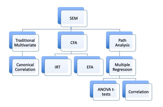
Relation to EFA
- You have a bunch of questions
- You have an idea (or sometimes not!) of how many factors to expect
- You let the questions go where they want
- You remove the bad questions until you get a good fit
CFA models
- You set up the model with specific questions onto specific factors
- Forcing the cross loadings be zero
- You test to see if that model fits
- So, you may think about how confirmatory factor analysis is step two to exploring (exploratory factor analysis)
CFA Models
- Reflective – the latent variable causes the manifest variables scores
- Purpose is to understand the relationships between the measured variables
- Same theoretical concept as EFA
CFA Models Reflective Example
# a famous example, build the model
HS.model <- ' visual  =~ x1 + x2 + x3
              textual =~ x4 + x5 + x6
              speed   =~ x7 + x8 + x9 '

# fit the model
HS.fit <- cfa(HS.model, data = HolzingerSwineford1939)

# diagram the model
semPaths(HS.fit,
         whatLabels = "std",
         layout = "tree",
         edge.label.cex = 1)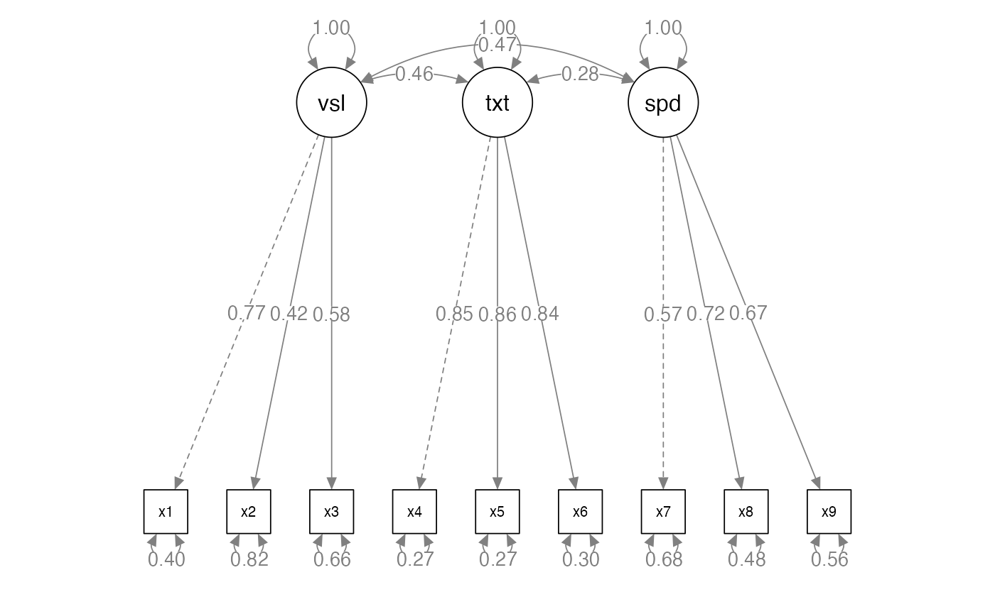
CFA Models
- Formative – latent variables are the result of manifest variables
- Similar to principal components analysis theoretical concept
- Potentially a use for demographics?
CFA Models Formative Example
# a famous example, build the model
HS.model <- ' visual  <~ x1 + x2 + x3'

# fit the model
HS.fit <- cfa(HS.model, data = HolzingerSwineford1939)
#> Warning: lavaan->lav_data_full():
#>    all observed variables are exogenous; model may not be identified
#> Warning: lavaan->lav_model_vcov():
#>    Could not compute standard errors! The information matrix could not be
#>    inverted. This may be a symptom that the model is not identified.

# diagram the model
semPaths(HS.fit,
         whatLabels = "std",
         layout = "tree",
         edge.label.cex = 1)
CFA Models
- The manifest variables in a CFA are sometimes called indicator variables
- Because they indicate what the latent variable should be since we do not directly measure the latent variable
General Set Up
- The latents will be correlated (because they are exogenous only)
- Similar to an oblique rotation
- Each factor section has to be identified
- You should have three measured variables per latent
- If you only have two, you need to set their coefficients to equal (estimated but equal)
- Arrows go from latent to measured (reflexive)
- We think that latent caused the measured answers
- Error terms on the measured variables, variance on the latent
variables
- If you are counting for degrees of freedom for identification
Correlated Error
- Generally, you leave the error terms uncorrelated, as you think they are separate items
- However:
- These questions all measure the same factor right?
- Often they are pretty similar
- Some answers will be related to other items
- So it’s not too big of a idea to say that item’s errors are related
- We can use modification indices to see if they should be correlated
- Make sure these make sense!
Interpretation
- The latent variable section includes the
factor loadingsor coefficients - These are the same idea as EFA - you want the relationship between
the latent variable and the manifest variable to be strong
- We used a rule of .300 before but for this rule, you should examine the standardized loading
- Otherwise, why would we think this item measures the latent variable?
Interpretation
- These coefficients are often called:
- Pattern coefficients (unstandardized): for every one unit in the latent variable, the manifest variable increases b units
- Structure coefficients (standardized): the correlation between the latent variable and the manifest variable
Identification Rules of Thumb:
- Latent variables should have four indicators
- Latent variables have three indicators AND error variances do not covary
- Latent variables have two indicators AND Error variances do not covary AND loadings are set to equal each other
Scaling
- Remember that scaling is the way we “set the scale” for the latent variable
- We usually do this by setting one of the pattern coefficients to 1 - the marker variable approach
- Another option is to to set the variance of the latent variable to 1
std.lvin the the standardized output- What does that do?
- Sets the scale to z-score
- Makes double headed arrow between latents correlation
- Make sure you are using unstandardized data!
Scaling
- So what is the
std.allas part of the “completely standardized solution? - Both the latent variable variance and the manifest variable variance is set to 1
- If you are going to report the standardized solution, this version is the most common, as it matches EFA and regression
- All of these options give you different loadings, but should not change model fit
Examples
- Reminder:
- When you use a correlation matrix as your input, the solution is already standardized!
- When you use a covariance matrix as your input, both the unstandardized and standardized solution can be viewed
One-Factor CFA Example
- IQ is often thought of as “g” or this overall cognitive ability
- Let’s look at an example of the WISC, which is an IQ test for children
- We have five of the subtest scores including
information,similarities,word reasoning,matrix reasoning, andpicture concepts
Convert Correlations to Covariance
wisc4.cor <- lav_matrix_lower2full(c(1,
                                     0.72,1,
                                     0.64,0.63,1,
                                     0.51,0.48,0.37,1,
                                     0.37,0.38,0.38,0.38,1))
# enter the SDs
wisc4.sd <- c(3.01 , 3.03 , 2.99 , 2.89 , 2.98)

# give everything names
colnames(wisc4.cor) <-
  rownames(wisc4.cor) <-
  names(wisc4.sd) <-
  c("Information", "Similarities",
    "Word.Reasoning", "Matrix.Reasoning", "Picture.Concepts")

# convert
wisc4.cov <- cor2cov(wisc4.cor, wisc4.sd)
WISC One-Factor Model
- The
=~is used to define a reflexive latent variable -
~can be interpreted as Y is predicted by X -
=~can be interpreted as X is indicated by Ys
wisc4.model <- '
g =~ Information + Similarities + Word.Reasoning + Matrix.Reasoning + Picture.Concepts
'
Analyze the Model
- Notice we changed to the
cfa()function - It has the same basic arguments
- The
std.lvoption can be used to only see the standardized solution on the latent variable, usually you want to set this toFALSE
wisc4.fit <- cfa(model = wisc4.model,
                sample.cov = wisc4.cov,
                sample.nobs = 550,
                std.lv = FALSE)
Summarize the Model
- Logical solution:
- Positive variances
- SMCs + Correlations < 1
- No error messages
- SEs are not “huge”
- Estimates:
- Do our questions load appropriately?
- Model fit:
- What do the fit indices indicate?
- Can we improve model fit without overfitting?
Summarize the Model
summary(wisc4.fit,
        standardized=TRUE,
        rsquare = TRUE,
        fit.measures=TRUE)
#> lavaan 0.6-19 ended normally after 30 iterations
#>
#>   Estimator                                         ML
#>   Optimization method                           NLMINB
#>   Number of model parameters                        10
#>
#>   Number of observations                           550
#>
#> Model Test User Model:
#>
#>   Test statistic                                26.775
#>   Degrees of freedom                                 5
#>   P-value (Chi-square)                           0.000
#>
#> Model Test Baseline Model:
#>
#>   Test statistic                              1073.427
#>   Degrees of freedom                                10
#>   P-value                                        0.000
#>
#> User Model versus Baseline Model:
#>
#>   Comparative Fit Index (CFI)                    0.980
#>   Tucker-Lewis Index (TLI)                       0.959
#>
#> Loglikelihood and Information Criteria:
#>
#>   Loglikelihood user model (H0)              -6378.678
#>   Loglikelihood unrestricted model (H1)      -6365.291
#>
#>   Akaike (AIC)                               12777.357
#>   Bayesian (BIC)                             12820.456
#>   Sample-size adjusted Bayesian (SABIC)      12788.712
#>
#> Root Mean Square Error of Approximation:
#>
#>   RMSEA                                          0.089
#>   90 Percent confidence interval - lower         0.058
#>   90 Percent confidence interval - upper         0.123
#>   P-value H_0: RMSEA <= 0.050                    0.022
#>   P-value H_0: RMSEA >= 0.080                    0.708
#>
#> Standardized Root Mean Square Residual:
#>
#>   SRMR                                           0.034
#>
#> Parameter Estimates:
#>
#>   Standard errors                             Standard
#>   Information                                 Expected
#>   Information saturated (h1) model          Structured
#>
#> Latent Variables:
#>                    Estimate  Std.Err  z-value  P(>|z|)   Std.lv  Std.all
#>   g =~
#>     Information       1.000                               2.578    0.857
#>     Similarities      0.985    0.045   21.708    0.000    2.541    0.839
#>     Word.Reasoning    0.860    0.045   18.952    0.000    2.217    0.742
#>     Matrix.Reasnng    0.647    0.047   13.896    0.000    1.669    0.578
#>     Picture.Cncpts    0.542    0.050   10.937    0.000    1.398    0.470
#>
#> Variances:
#>                    Estimate  Std.Err  z-value  P(>|z|)   Std.lv  Std.all
#>    .Information       2.395    0.250    9.587    0.000    2.395    0.265
#>    .Similarities      2.709    0.258   10.482    0.000    2.709    0.296
#>    .Word.Reasoning    4.009    0.295   13.600    0.000    4.009    0.449
#>    .Matrix.Reasnng    5.551    0.360   15.400    0.000    5.551    0.666
#>    .Picture.Cncpts    6.909    0.434   15.922    0.000    6.909    0.779
#>     g                 6.648    0.564   11.788    0.000    1.000    1.000
#>
#> R-Square:
#>                    Estimate
#>     Information       0.735
#>     Similarities      0.704
#>     Word.Reasoning    0.551
#>     Matrix.Reasnng    0.334
#>     Picture.Cncpts    0.221
New Functions
-
std.nox: the standardized estimates are based on both the variances of both (continuous) observed and latent variables, but not the variances of exogenous covariates - This output is the best way to get the confidence intervals for each parameter
parameterestimates(wisc4.fit,
                   standardized=TRUE)
#>                 lhs op              rhs   est    se      z pvalue ci.lower
#> 1                 g =~      Information 1.000 0.000     NA     NA    1.000
#> 2                 g =~     Similarities 0.985 0.045 21.708      0    0.896
#> 3                 g =~   Word.Reasoning 0.860 0.045 18.952      0    0.771
#> 4                 g =~ Matrix.Reasoning 0.647 0.047 13.896      0    0.556
#> 5                 g =~ Picture.Concepts 0.542 0.050 10.937      0    0.445
#> 6       Information ~~      Information 2.395 0.250  9.587      0    1.906
#> 7      Similarities ~~     Similarities 2.709 0.258 10.482      0    2.202
#> 8    Word.Reasoning ~~   Word.Reasoning 4.009 0.295 13.600      0    3.431
#> 9  Matrix.Reasoning ~~ Matrix.Reasoning 5.551 0.360 15.400      0    4.845
#> 10 Picture.Concepts ~~ Picture.Concepts 6.909 0.434 15.922      0    6.058
#> 11                g ~~                g 6.648 0.564 11.788      0    5.543
#>    ci.upper std.lv std.all
#> 1     1.000  2.578   0.857
#> 2     1.074  2.541   0.839
#> 3     0.949  2.217   0.742
#> 4     0.739  1.669   0.578
#> 5     0.640  1.398   0.470
#> 6     2.885  2.395   0.265
#> 7     3.215  2.709   0.296
#> 8     4.587  4.009   0.449
#> 9     6.258  5.551   0.666
#> 10    7.759  6.909   0.779
#> 11    7.754  1.000   1.000
New Functions
fitted(wisc4.fit) ## estimated covariances
#> $cov
#>                  Infrmt Smlrts Wrd.Rs Mtrx.R Pctr.C
#> Information       9.044
#> Similarities      6.551  9.164
#> Word.Reasoning    5.716  5.633  8.924
#> Matrix.Reasoning  4.303  4.241  3.700  8.337
#> Picture.Concepts  3.606  3.553  3.100  2.334  8.864
wisc4.cov ## actual covariances
#>                  Information Similarities Word.Reasoning Matrix.Reasoning
#> Information         9.060100     6.566616       5.759936         4.436439
#> Similarities        6.566616     9.180900       5.707611         4.203216
#> Word.Reasoning      5.759936     5.707611       8.940100         3.197207
#> Matrix.Reasoning    4.436439     4.203216       3.197207         8.352100
#> Picture.Concepts    3.318826     3.431172       3.385876         3.272636
#>                  Picture.Concepts
#> Information              3.318826
#> Similarities             3.431172
#> Word.Reasoning           3.385876
#> Matrix.Reasoning         3.272636
#> Picture.Concepts         8.880400
All Fit Indices
fitmeasures(wisc4.fit)
#>                  npar                  fmin                 chisq
#>                10.000                 0.024                26.775
#>                    df                pvalue        baseline.chisq
#>                 5.000                 0.000              1073.427
#>           baseline.df       baseline.pvalue                   cfi
#>                10.000                 0.000                 0.980
#>                   tli                  nnfi                   rfi
#>                 0.959                 0.959                 0.950
#>                   nfi                  pnfi                   ifi
#>                 0.975                 0.488                 0.980
#>                   rni                  logl     unrestricted.logl
#>                 0.980             -6378.678             -6365.291
#>                   aic                   bic                ntotal
#>             12777.357             12820.456               550.000
#>                  bic2                 rmsea        rmsea.ci.lower
#>             12788.712                 0.089                 0.058
#>        rmsea.ci.upper        rmsea.ci.level          rmsea.pvalue
#>                 0.123                 0.900                 0.022
#>        rmsea.close.h0 rmsea.notclose.pvalue     rmsea.notclose.h0
#>                 0.050                 0.708                 0.080
#>                   rmr            rmr_nomean                  srmr
#>                 0.298                 0.298                 0.034
#>          srmr_bentler   srmr_bentler_nomean                  crmr
#>                 0.034                 0.034                 0.042
#>           crmr_nomean            srmr_mplus     srmr_mplus_nomean
#>                 0.042                 0.034                 0.034
#>                 cn_05                 cn_01                   gfi
#>               228.408               310.899                 0.982
#>                  agfi                  pgfi                   mfi
#>                 0.947                 0.327                 0.980
#>                  ecvi
#>                 0.085
Modification Indices
modificationindices(wisc4.fit, sort = T)
#>                 lhs op              rhs     mi    epc sepc.lv sepc.all sepc.nox
#> 21 Matrix.Reasoning ~~ Picture.Concepts 14.157  1.058   1.058    0.171    0.171
#> 19   Word.Reasoning ~~ Matrix.Reasoning  8.931 -0.710  -0.710   -0.151   -0.151
#> 15      Information ~~ Picture.Concepts  5.493 -0.565  -0.565   -0.139   -0.139
#> 20   Word.Reasoning ~~ Picture.Concepts  2.029  0.365   0.365    0.069    0.069
#> 14      Information ~~ Matrix.Reasoning  1.447  0.280   0.280    0.077    0.077
#> 18     Similarities ~~ Picture.Concepts  0.838 -0.223  -0.223   -0.051   -0.051
#> 16     Similarities ~~   Word.Reasoning  0.791  0.242   0.242    0.073    0.073
#> 13      Information ~~   Word.Reasoning  0.279  0.147   0.147    0.047    0.047
#> 17     Similarities ~~ Matrix.Reasoning  0.147 -0.089  -0.089   -0.023   -0.023
#> 12      Information ~~     Similarities  0.010  0.034   0.034    0.013    0.013
Diagram the Model
semPaths(wisc4.fit,
         whatLabels="std",
         what = "std",
         layout ="tree",
         edge.color = "blue",
         edge.label.cex = 1)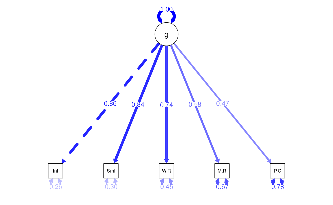
WISC Two-Factor Model
- Note that we only have two items on the latent variable
- If we see an identification error, we can set these to equal (homework hint!)
wisc4.model2 <- '
V =~ Information + Similarities + Word.Reasoning
F =~ Matrix.Reasoning + Picture.Concepts
'

# wisc4.model2 <- '
# V =~ Information + Similarities + Word.Reasoning
# F =~ a*Matrix.Reasoning + a*Picture.Concepts
# '
Analyze the Model
wisc4.fit2 <- cfa(wisc4.model2,
                  sample.cov=wisc4.cov,
                  sample.nobs=550,
                  std.lv = F)
Summarize the Model
summary(wisc4.fit2,
        standardized=TRUE,
        rsquare = TRUE,
        fit.measures=TRUE)
#> lavaan 0.6-19 ended normally after 44 iterations
#>
#>   Estimator                                         ML
#>   Optimization method                           NLMINB
#>   Number of model parameters                        11
#>
#>   Number of observations                           550
#>
#> Model Test User Model:
#>
#>   Test statistic                                12.687
#>   Degrees of freedom                                 4
#>   P-value (Chi-square)                           0.013
#>
#> Model Test Baseline Model:
#>
#>   Test statistic                              1073.427
#>   Degrees of freedom                                10
#>   P-value                                        0.000
#>
#> User Model versus Baseline Model:
#>
#>   Comparative Fit Index (CFI)                    0.992
#>   Tucker-Lewis Index (TLI)                       0.980
#>
#> Loglikelihood and Information Criteria:
#>
#>   Loglikelihood user model (H0)              -6371.634
#>   Loglikelihood unrestricted model (H1)      -6365.291
#>
#>   Akaike (AIC)                               12765.269
#>   Bayesian (BIC)                             12812.678
#>   Sample-size adjusted Bayesian (SABIC)      12777.759
#>
#> Root Mean Square Error of Approximation:
#>
#>   RMSEA                                          0.063
#>   90 Percent confidence interval - lower         0.026
#>   90 Percent confidence interval - upper         0.103
#>   P-value H_0: RMSEA <= 0.050                    0.244
#>   P-value H_0: RMSEA >= 0.080                    0.272
#>
#> Standardized Root Mean Square Residual:
#>
#>   SRMR                                           0.019
#>
#> Parameter Estimates:
#>
#>   Standard errors                             Standard
#>   Information                                 Expected
#>   Information saturated (h1) model          Structured
#>
#> Latent Variables:
#>                    Estimate  Std.Err  z-value  P(>|z|)   Std.lv  Std.all
#>   V =~
#>     Information       1.000                               2.587    0.860
#>     Similarities      0.984    0.046   21.625    0.000    2.545    0.841
#>     Word.Reasoning    0.858    0.045   18.958    0.000    2.219    0.743
#>   F =~
#>     Matrix.Reasnng    1.000                               1.989    0.689
#>     Picture.Cncpts    0.825    0.085    9.747    0.000    1.642    0.552
#>
#> Covariances:
#>                    Estimate  Std.Err  z-value  P(>|z|)   Std.lv  Std.all
#>   V ~~
#>     F                 4.233    0.399   10.604    0.000    0.823    0.823
#>
#> Variances:
#>                    Estimate  Std.Err  z-value  P(>|z|)   Std.lv  Std.all
#>    .Information       2.352    0.253    9.295    0.000    2.352    0.260
#>    .Similarities      2.685    0.261   10.282    0.000    2.685    0.293
#>    .Word.Reasoning    4.000    0.295   13.555    0.000    4.000    0.448
#>    .Matrix.Reasnng    4.380    0.458    9.557    0.000    4.380    0.525
#>    .Picture.Cncpts    6.168    0.451   13.673    0.000    6.168    0.696
#>     V                 6.692    0.567   11.807    0.000    1.000    1.000
#>     F                 3.957    0.569    6.960    0.000    1.000    1.000
#>
#> R-Square:
#>                    Estimate
#>     Information       0.740
#>     Similarities      0.707
#>     Word.Reasoning    0.552
#>     Matrix.Reasnng    0.475
#>     Picture.Cncpts    0.304
Diagram the Model
semPaths(wisc4.fit2,
         whatLabels="std",
         what = "std",
         edge.color = "pink",
         edge.label.cex = 1,
         layout="tree")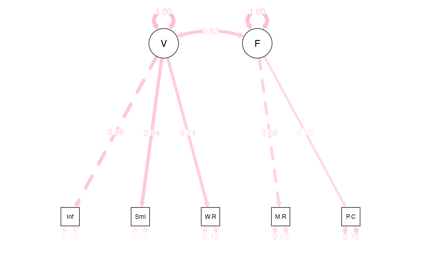
Compare the Models
anova(wisc4.fit, wisc4.fit2)
#>
#> Chi-Squared Difference Test
#>
#>            Df   AIC   BIC  Chisq Chisq diff   RMSEA Df diff Pr(>Chisq)
#> wisc4.fit2  4 12765 12813 12.687
#> wisc4.fit   5 12777 12820 26.775     14.088 0.15426       1  0.0001745 ***
#> ---
#> Signif. codes:  0 '***' 0.001 '**' 0.01 '*' 0.05 '.' 0.1 ' ' 1
fitmeasures(wisc4.fit, c("aic", "ecvi"))
#>       aic      ecvi
#> 12777.357     0.085
fitmeasures(wisc4.fit2, c("aic", "ecvi"))
#>       aic      ecvi
#> 12765.269     0.063
How to Tidy lavaan Output
#install.packages("parameters")
library(parameters)
model_parameters(wisc4.fit, standardize = TRUE)
#> # Loading
#>
#> Link                  | Coefficient |   SE |       95% CI |     z |      p
#> --------------------------------------------------------------------------
#> g =~ Information      |        0.86 | 0.02 | [0.82, 0.89] | 49.47 | < .001
#> g =~ Similarities     |        0.84 | 0.02 | [0.80, 0.87] | 46.32 | < .001
#> g =~ Word.Reasoning   |        0.74 | 0.02 | [0.70, 0.79] | 32.26 | < .001
#> g =~ Matrix.Reasoning |        0.58 | 0.03 | [0.52, 0.64] | 18.29 | < .001
#> g =~ Picture.Concepts |        0.47 | 0.04 | [0.40, 0.54] | 12.94 | < .001
How to Tidy lavaan Output
library(broom)
tidy(wisc4.fit)
#> # A tibble: 11 × 8
#>    term                op    estimate std.error statistic p.value std.lv std.all
#>    <chr>               <chr>    <dbl>     <dbl>     <dbl>   <dbl>  <dbl>   <dbl>
#>  1 g =~ Information    =~       1        0          NA         NA   2.58   0.857
#>  2 g =~ Similarities   =~       0.985    0.0454     21.7        0   2.54   0.839
#>  3 g =~ Word.Reasoning =~       0.860    0.0454     19.0        0   2.22   0.742
#>  4 g =~ Matrix.Reason… =~       0.647    0.0466     13.9        0   1.67   0.578
#>  5 g =~ Picture.Conce… =~       0.542    0.0496     10.9        0   1.40   0.470
#>  6 Information ~~ Inf… ~~       2.40     0.250       9.59       0   2.40   0.265
#>  7 Similarities ~~ Si… ~~       2.71     0.258      10.5        0   2.71   0.296
#>  8 Word.Reasoning ~~ … ~~       4.01     0.295      13.6        0   4.01   0.449
#>  9 Matrix.Reasoning ~… ~~       5.55     0.360      15.4        0   5.55   0.666
#> 10 Picture.Concepts ~… ~~       6.91     0.434      15.9        0   6.91   0.779
#> 11 g ~~ g              ~~       6.65     0.564      11.8        0   1      1
glance(wisc4.fit)
#> # A tibble: 1 × 17
#>    agfi    AIC    BIC   cfi chisq  npar  rmsea rmsea.conf.high   srmr   tli
#>   <dbl>  <dbl>  <dbl> <dbl> <dbl> <dbl>  <dbl>           <dbl>  <dbl> <dbl>
#> 1 0.947 12777. 12820. 0.980  26.8    10 0.0890           0.123 0.0345 0.959
#> # ℹ 7 more variables: converged <lgl>, estimator <chr>, ngroups <int>,
#> #   missing_method <chr>, nobs <dbl>, norig <dbl>, nexcluded <dbl>