Path Analysis • learnSEM

Estimation

Estimation is the math that goes on behind the scenes to give you parameter numbers
Common types:
- Maximum Likelihood (ML)
- Asymptotically Distribution Free (ADF)
- Unweighted Least Squares (ULS)
- Two stage least squares (TSLS)

Maximum Likelihood

Estimates are the ones that maximize the likelihood that the data were drawn from the population
Normal theory method - multivariate normality is assumed to use ML
- Check your normality assumption!
- Other types of estimations may work better for non-normal endogenous variables
Full information method - estimates are calculated all at the same time
- Partial information methods calculate part of the estimates, then use those to calculate the rest

Maximum Likelihood

Fit function - the relationship between the sample covariances and estimated covariances
We want our fit function to be:
- High if we are measuring how much they match (goodness of fit)
- Low if we are measuring how much they mismatch (residuals)

Maximum Likelihood

ML is an iterative process
The computer calculates a possible start solution
Then runs several times to create the largest ML match
Start values:
- Usually generated by the computer
- You can enter values if you are having problems converging to a solution

Maximum Likelihood

Scale free/invariant
- Means that if you change the scale with a linear transform, the model is still the same
Assumes unstandardized start variables
- Otherwise you would be standardizing standardized estimates
Interpretation of Estimates
- Loadings/path coefficients - just like regression coefficients
- Covariance/correlation - how much two items vary together
- Error variances tell you how much variance is not accounted for by the model (so you want to be small)
- SMCs are the amount of variance accounted for in a endogenous variable

Other Methods

For continuous variables with normal distributions:
- Generalized Least Squares (GLS)
- Unweighted Least Squares (ULS)
- Fully Weighted Least Squares (WLS)

Generalized Least Squares

Pros:
- Scale free
- Faster computation time
Cons:
- Not commonly used? If this runs usually so does ML

Unweighted Least Squares

Pros:
- Does not require positive definite matrices
- Robust initial estimates
Cons:
- Not scale free
- Not as efficient
- All variables in the same scale

Other Methods

Nonnormal data
- In ML, estimates might be accurate but standard errors may be large
- Model fit tends to be overestimated
Corrected normal method - uses ML but then adjusts the SEs to be normal (robust SE).
- Satorra-Bentler statistic: Adjusts the chi square value from standard ML by the degree of kurtosis/skew
- Corrected model test statistic

Asymptotically Distribution Free

Some books call this arbitrary distribution free
Estimates the skew/kurtosis in the data to generate a model
May not converge because of number of parameters to estimate

Errors

Inadmissible solutions - you get numbers in your output but clearly parameters are
Heywood cases
- Parameter estimates are illogical (huge)
- Negative variance estimates
  - Just variances, covariances can be negative
- Correlation estimates over 1 (SMCs)

Why Errors Happen

Specification error
Nonidentification
Outliers
Small samples
Two indicators per latent (more is always better)
Bad start values (especially for errors)
Very low or high correlations (empirical under identification)

Path Models

Reminder:
- Circles are latent (unobserved) variables
- Squares are manifest (observed) variables
- Triangles can be used to represent intercepts (specific models use these)
So what is a path model?
- A model with only manifest variables (measured/squares)

Path Models

Straight arrows are “causal” or directional
- Non-standardized solution -> these are your b or slope values
- Standardized solution -> these are your beta values
Curved arrows are non-directional
- Non-standardized -> covariance
- Standardized -> correlation

Path Models

All endogenous variables have an error term
All exogenous variables will have a variance
All exogenous only variables are automatically correlated by lavaan

Solutions

Why standardized?
- Allows you to compare path coefficients for strength of relationship
- Makes the non-directional relationships correlation (more interpretable)
- Matches the values you are used to thinking about (EFA)
Why unstandardized?
- Allows you to estimate future scores and interpret path coefficients, in the original scale of the data

Let’s do it!

Install lavaan: latent variable analysis
Install semPlot: helps us make pictures

install.packages("lavaan")
install.packages("semPlot")

Syntax

Note: there’s a cheat sheet guide on Canvas
First, we will define a “model”
- Best practice: name the saved variable something like name.model where name is a descriptive name of the model you are building
Model syntax
- ~ indicates a regression
- ~~ indicates a covariance/correlation
- =~ indicates a latent variable

Syntax

Automatically adds an error term to each endogenous variable
Automatically constrains the path to 1 for you for the marker variable
Automatically adds a covariance term between all exogenous variables
- Very useful for analyses we will get to later
- Not always required in path models, but you could constrain it to zero
- Important to note because it’s often unexpected

A Path Example

library(rio)
eval.data <- import("data/lecture_evals.csv")

A Path Example

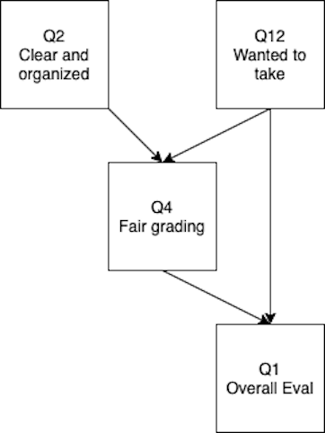
Estimate df

Possible = $\frac{4 \times (4+1)}{2} = 10$
Estimated:
- 4 regressions
- 2 error variances
- 2 variances
- 1 covariance
DF = 10 - 9 = 1

Build the model

library(lavaan)
#> This is lavaan 0.6-19
#> lavaan is FREE software! Please report any bugs.
eval.model <- '
q4 ~ q12 + q2
q1 ~ q4 + q12
'

Important Notes

eval.model
#> [1] "\nq4 ~ q12 + q2\nq1 ~ q4 + q12\n"

Note that \n is code for new lines
- These are important
- Spacing is not important
- You can use # in the code, it will ignore that line just like R

Run the Model

We can use the sem() function to apply the model to the data
Save the analysis, use good naming like eval.output
The default estimator is normal theory maximum likelihood
Use ?sem to learn more about the options

eval.output <- sem(model = eval.model,
                   data = eval.data)

View the Output

summary(eval.output)
#> lavaan 0.6-19 ended normally after 2 iterations
#> 
#>   Estimator                                         ML
#>   Optimization method                           NLMINB
#>   Number of model parameters                         6
#> 
#>   Number of observations                          3585
#> 
#> Model Test User Model:
#>                                                       
#>   Test statistic                              2152.922
#>   Degrees of freedom                                 1
#>   P-value (Chi-square)                           0.000
#> 
#> Parameter Estimates:
#> 
#>   Standard errors                             Standard
#>   Information                                 Expected
#>   Information saturated (h1) model          Structured
#> 
#> Regressions:
#>                    Estimate  Std.Err  z-value  P(>|z|)
#>   q4 ~                                                
#>     q12               0.096    0.008   12.479    0.000
#>     q2                0.435    0.010   45.655    0.000
#>   q1 ~                                                
#>     q4                0.840    0.017   49.923    0.000
#>     q12               0.263    0.010   26.551    0.000
#> 
#> Variances:
#>                    Estimate  Std.Err  z-value  P(>|z|)
#>    .q4                0.094    0.002   42.338    0.000
#>    .q1                0.151    0.004   42.338    0.000

Output

Default output includes:
- Sample size
- Estimator
- Minimum function test statistic $\chi^2$ , df, p
- Unstandardized parameter estimates, standard error, Z, p

Improved Output

summary(eval.output, 
        standardized = TRUE, # for the standardized solution
        fit.measures = TRUE, # for model fit
        rsquare = TRUE) # for SMCs
#> lavaan 0.6-19 ended normally after 2 iterations
#> 
#>   Estimator                                         ML
#>   Optimization method                           NLMINB
#>   Number of model parameters                         6
#> 
#>   Number of observations                          3585
#> 
#> Model Test User Model:
#>                                                       
#>   Test statistic                              2152.922
#>   Degrees of freedom                                 1
#>   P-value (Chi-square)                           0.000
#> 
#> Model Test Baseline Model:
#> 
#>   Test statistic                              7293.347
#>   Degrees of freedom                                 5
#>   P-value                                        0.000
#> 
#> User Model versus Baseline Model:
#> 
#>   Comparative Fit Index (CFI)                    0.705
#>   Tucker-Lewis Index (TLI)                      -0.476
#> 
#> Loglikelihood and Information Criteria:
#> 
#>   Loglikelihood user model (H0)              -2539.494
#>   Loglikelihood unrestricted model (H1)      -1463.033
#>                                                       
#>   Akaike (AIC)                                5090.988
#>   Bayesian (BIC)                              5128.095
#>   Sample-size adjusted Bayesian (SABIC)       5109.030
#> 
#> Root Mean Square Error of Approximation:
#> 
#>   RMSEA                                          0.775
#>   90 Percent confidence interval - lower         0.747
#>   90 Percent confidence interval - upper         0.802
#>   P-value H_0: RMSEA <= 0.050                    0.000
#>   P-value H_0: RMSEA >= 0.080                    1.000
#> 
#> Standardized Root Mean Square Residual:
#> 
#>   SRMR                                           0.105
#> 
#> Parameter Estimates:
#> 
#>   Standard errors                             Standard
#>   Information                                 Expected
#>   Information saturated (h1) model          Structured
#> 
#> Regressions:
#>                    Estimate  Std.Err  z-value  P(>|z|)   Std.lv  Std.all
#>   q4 ~                                                                  
#>     q12               0.096    0.008   12.479    0.000    0.096    0.164
#>     q2                0.435    0.010   45.655    0.000    0.435    0.598
#>   q1 ~                                                                  
#>     q4                0.840    0.017   49.923    0.000    0.840    0.585
#>     q12               0.263    0.010   26.551    0.000    0.263    0.311
#> 
#> Variances:
#>                    Estimate  Std.Err  z-value  P(>|z|)   Std.lv  Std.all
#>    .q4                0.094    0.002   42.338    0.000    0.094    0.553
#>    .q1                0.151    0.004   42.338    0.000    0.151    0.431
#> 
#> R-Square:
#>                    Estimate
#>     q4                0.447
#>     q1                0.569

Create a Picture

Sometimes it’s hard to know if you have modeled what you intended to diagram
Let’s create a plot to make sure it’s what we meant to do

library(semPlot)
semPaths(eval.output, # the analyzed model 
         whatLabels = "par", # what to add as the numbers, std for standardized
         edge.label.cex = 1, # make the font bigger
         layout = "spring") # change the layout tree, circle, spring, tree2, circle2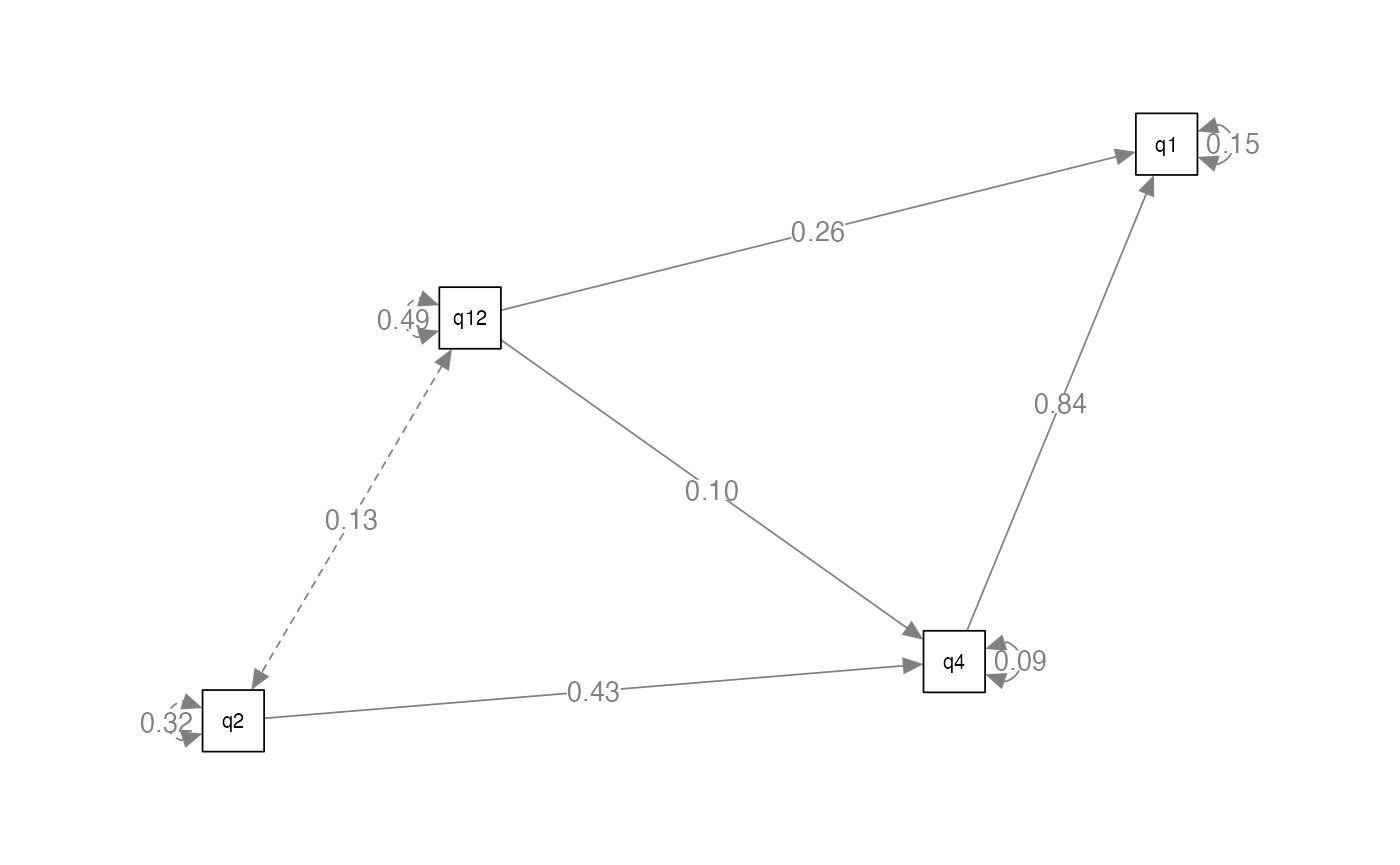

Another Example

You don’t actually have to have the data to run an analysis
If you have the correlation matrix, you can still run the analysis
It’s always better to use the raw data if you have it!

regression.cor <- lav_matrix_lower2full(c(1.00,
                                         0.20,1.00,
                                         0.24,0.30,1.00,
                                         0.70,0.80,0.30,1.00))

# name the variables in the matrix
colnames(regression.cor) <-
  rownames(regression.cor) <-
  c("X1", "X2", "X3", "Y")

Build the Model

Let’s look at how we can label the paths

regression.model <- '
# structural model for Y
Y ~ a*X1 + b*X2 + c*X3 
# label the residual variance of Y
Y ~~ z*Y 
'

Analyze the Model

regression.fit <- sem(model = regression.model,
                      sample.cov = regression.cor, # instead of data
                      sample.nobs = 1000) # number of data points

View the Summary

summary(regression.fit, 
        standardized = TRUE,
        fit.measures = TRUE,
        rsquare = TRUE)
#> lavaan 0.6-19 ended normally after 1 iteration
#> 
#>   Estimator                                         ML
#>   Optimization method                           NLMINB
#>   Number of model parameters                         4
#> 
#>   Number of observations                          1000
#> 
#> Model Test User Model:
#>                                                       
#>   Test statistic                                 0.000
#>   Degrees of freedom                                 0
#> 
#> Model Test Baseline Model:
#> 
#>   Test statistic                              2913.081
#>   Degrees of freedom                                 3
#>   P-value                                        0.000
#> 
#> User Model versus Baseline Model:
#> 
#>   Comparative Fit Index (CFI)                    1.000
#>   Tucker-Lewis Index (TLI)                       1.000
#> 
#> Loglikelihood and Information Criteria:
#> 
#>   Loglikelihood user model (H0)                 38.102
#>   Loglikelihood unrestricted model (H1)         38.102
#>                                                       
#>   Akaike (AIC)                                 -68.205
#>   Bayesian (BIC)                               -48.574
#>   Sample-size adjusted Bayesian (SABIC)        -61.278
#> 
#> Root Mean Square Error of Approximation:
#> 
#>   RMSEA                                          0.000
#>   90 Percent confidence interval - lower         0.000
#>   90 Percent confidence interval - upper         0.000
#>   P-value H_0: RMSEA <= 0.050                       NA
#>   P-value H_0: RMSEA >= 0.080                       NA
#> 
#> Standardized Root Mean Square Residual:
#> 
#>   SRMR                                           0.000
#> 
#> Parameter Estimates:
#> 
#>   Standard errors                             Standard
#>   Information                                 Expected
#>   Information saturated (h1) model          Structured
#> 
#> Regressions:
#>                    Estimate  Std.Err  z-value  P(>|z|)   Std.lv  Std.all
#>   Y ~                                                                   
#>     X1         (a)    0.571    0.008   74.539    0.000    0.571    0.571
#>     X2         (b)    0.700    0.008   89.724    0.000    0.700    0.700
#>     X3         (c)   -0.047    0.008   -5.980    0.000   -0.047   -0.047
#> 
#> Variances:
#>                    Estimate  Std.Err  z-value  P(>|z|)   Std.lv  Std.all
#>    .Y          (z)    0.054    0.002   22.361    0.000    0.054    0.054
#> 
#> R-Square:
#>                    Estimate
#>     Y                 0.946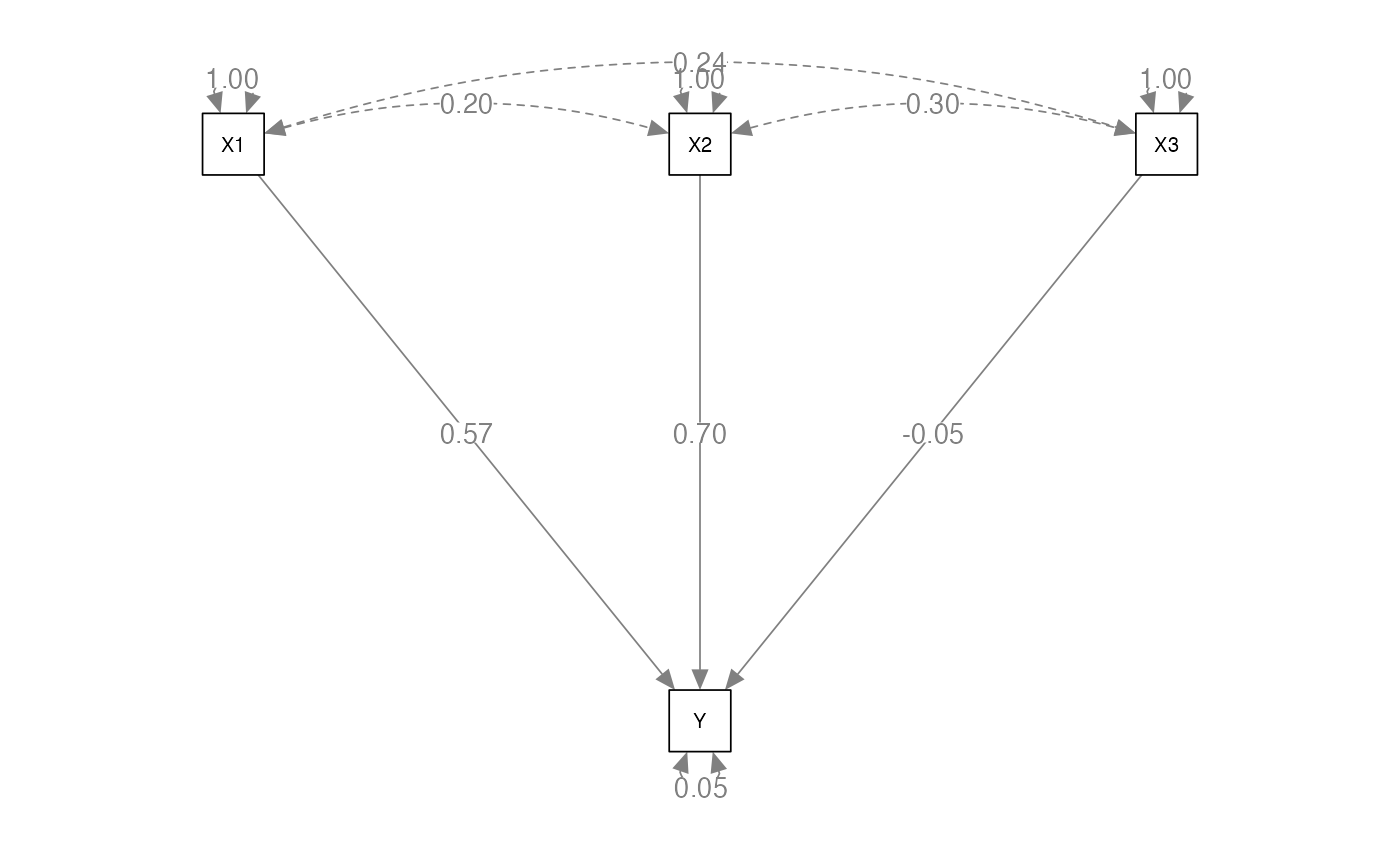

Create a Picture

semPaths(regression.fit, 
         whatLabels="par", 
         edge.label.cex = 1,
         layout="tree")

Mediation Models

Mediation models are regression models that imply that two variables are related (X and Y) until you add the mediator variable (M), which diminishes the relationship between X and Y
You can model these with regression or a structural layout

beaujean.cov <- lav_matrix_lower2full(c(648.07, 
                                        30.05, 8.64, 
                                        140.18, 25.57, 233.21))
colnames(beaujean.cov) <-
  rownames(beaujean.cov) <-
  c("salary", "school", "iq")

Build the Model

beaujean.model <- '
salary ~ a*school + c*iq
iq ~ b*school # this is reversed in first printing of the book 
ind:= b*c # this is the mediation part 
'

Analyze the Model

beaujean.fit <- sem(model = beaujean.model, 
                    sample.cov = beaujean.cov, 
                    sample.nobs = 300)

View the Summary

summary(beaujean.fit, 
        standardized = TRUE,
        fit.measures = TRUE,
        rsquare = TRUE)
#> lavaan 0.6-19 ended normally after 1 iteration
#> 
#>   Estimator                                         ML
#>   Optimization method                           NLMINB
#>   Number of model parameters                         5
#> 
#>   Number of observations                           300
#> 
#> Model Test User Model:
#>                                                       
#>   Test statistic                                 0.000
#>   Degrees of freedom                                 0
#> 
#> Model Test Baseline Model:
#> 
#>   Test statistic                               179.791
#>   Degrees of freedom                                 3
#>   P-value                                        0.000
#> 
#> User Model versus Baseline Model:
#> 
#>   Comparative Fit Index (CFI)                    1.000
#>   Tucker-Lewis Index (TLI)                       1.000
#> 
#> Loglikelihood and Information Criteria:
#> 
#>   Loglikelihood user model (H0)              -2549.357
#>   Loglikelihood unrestricted model (H1)      -2549.357
#>                                                       
#>   Akaike (AIC)                                5108.713
#>   Bayesian (BIC)                              5127.232
#>   Sample-size adjusted Bayesian (SABIC)       5111.375
#> 
#> Root Mean Square Error of Approximation:
#> 
#>   RMSEA                                          0.000
#>   90 Percent confidence interval - lower         0.000
#>   90 Percent confidence interval - upper         0.000
#>   P-value H_0: RMSEA <= 0.050                       NA
#>   P-value H_0: RMSEA >= 0.080                       NA
#> 
#> Standardized Root Mean Square Residual:
#> 
#>   SRMR                                           0.000
#> 
#> Parameter Estimates:
#> 
#>   Standard errors                             Standard
#>   Information                                 Expected
#>   Information saturated (h1) model          Structured
#> 
#> Regressions:
#>                    Estimate  Std.Err  z-value  P(>|z|)   Std.lv  Std.all
#>   salary ~                                                              
#>     school     (a)    2.515    0.549    4.585    0.000    2.515    0.290
#>     iq         (c)    0.325    0.106    3.081    0.002    0.325    0.195
#>   iq ~                                                                  
#>     school     (b)    2.959    0.247   12.005    0.000    2.959    0.570
#> 
#> Variances:
#>                    Estimate  Std.Err  z-value  P(>|z|)   Std.lv  Std.all
#>    .salary          525.128   42.877   12.247    0.000  525.128    0.813
#>    .iq              157.011   12.820   12.247    0.000  157.011    0.676
#> 
#> R-Square:
#>                    Estimate
#>     salary            0.187
#>     iq                0.324
#> 
#> Defined Parameters:
#>                    Estimate  Std.Err  z-value  P(>|z|)   Std.lv  Std.all
#>     ind               0.963    0.323    2.984    0.003    0.963    0.111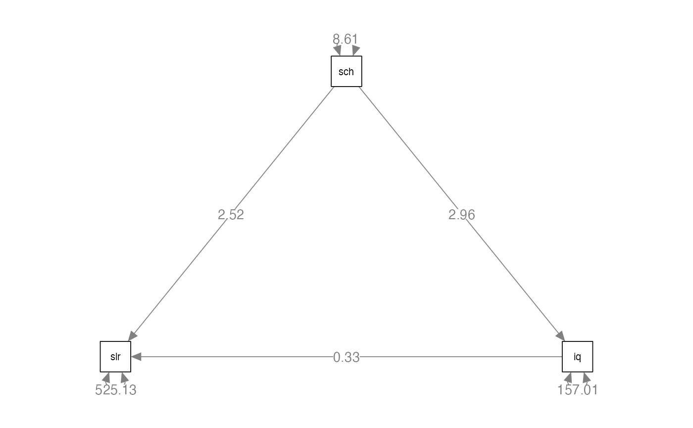

Create a Picture

semPaths(beaujean.fit, 
         whatLabels="par", 
         edge.label.cex = 1,
         layout="tree")

Fit Indices

Now that we’ve done a few examples, how can we know if our model is representative of the data?
We can use fit indices!
There are a lot of them
They do not imply that you are perfectly right
They have guidelines but they are not perfect either
People misuse them.

Limitations

Fit statistics indicate an overall/average model fit
That means there can be bad sections, but the overall fit is good
No one magical number/summary
They do not tell you where a misspecification occurs
Do not tell you the predictive value of a model
Do not tell you if it’s theoretically meaningful

“Rules”

Everyone cites Hu and Bentler (1999) for the golden standards.
Practically, these rules represent the same problems as rules about p values and effect sizes
Generally the rules fall into two categories:
- Goodness of fit statistics: want values close to 1
  - Excellent > .95, Good > .90
- Badness of fit statistics: want values close to 0
  - Excellent < .06, Good < .08, Acceptable < .10

Model Test Statistic

$\chi^2$
Examines if the reproduced correlation matrix matches the sample correlation matrix
Sometimes called “badness of fit”
You want this value to be small as it measures the “mismatch” or error

Model Test Statistic

Traditional null hypothesis testing reject-support context
- Generally, we reject the null to show that it’s unlikely, and therefore, the research hypothesis is likely
- However, here we want to support that the model represents the data, which is predicting the null
- So, it’s an odd use of $\chi^2$ to “support” the null

Model Test Statistic

χ2=(N−1)×FML\chi^2 = (N-1) \times FML
- FML is the minimum fit function in maximum likelihood estimation
- p values are based on the df for your model and the chi-square distribution
- You want this value to be non-significant (minus the issues of predicting the null)
- However, this non-significance is problematic!

Model Test Statistic

Chi-square is biased by:
- Multivariate non-normality
- Correlation size - large correlations can be hard to estimate
- Unique variance
- Sample size this is the big one

Model Test Statistic

Everyone reports chi-square, but people tend to ignore significant values
- One suggestion was normed chi-square $\frac{\chi^2}{df}$ - however, it is known to be just as problematic
Since χ2\chi^2 is biased, you could use a robust estimator to correct for bias
- Satorra-Bentler
- Yuan-Bentler

Alternative Fit Indices

There are three types of models:
- Your Model
- Independence - a model assuming no relationships between the variables (i.e., parameters are not significant)
- Saturated - a model assuming all parameters exist (i.e., df = 0).
We can use a ratio of your model compared to these other possible models as a way to determine fit.
These are less black and white, until we apply the “rules”
It’s easy to “cherry-pick” the best indices to support your model

Alternative Fit Indices

Absolute Fit Indices
Incremental Fit Indices
Parsimony-adjusted Indices
Predictive Fit Indices

Absolute fit indices

Proportion of the covariance matrix explained by the model
You can think about these as sort of $R^2$
Want these values be high
Goodness of Fit Index (GFI), Adjusted Goodness of Fit Index (AGFI), Parsimonious Goodness of Fit Index (PGFI)
- $1 - \frac{V_{residual}}{V_{total}}$
- Where residual is the variance not explained by the model, total is the total amount of variance
Research indicates these are positively biased, and they are not recommended for use

Absolute Fit Indices

Standardized root mean residual (SRMR)
Want small values, as it’s a badness of fit index

Incremental Fit Indices

Also known as comparative fit indices
- Values are to 0 to 1, want high values
Your model compared to the improvement over the independence model (no relationships)
Comparative Fit Index (CFI)
- $1 - \frac{\chi^2_{M} - df_{M}}{\chi^2_{B} - df_{B}}$
Normed Fit Index (NFI)
- A variation of the CFI, as it was said to underestimate for small samples
- $1 - \frac{\chi^2_{model}}{\chi^2_{baseline}}$

Incremental Fit Indices

Incremental Fit Index (IFI)
- Also known as Bollen’s Non-normed fit index
- Modified NFI that decreases emphasis on sample size
- $\frac{\chi^2_{baseline} - \chi^2_{model}}{\chi^2_{baseline} - df_{model}}$
Relative Fit Index (RFI)
- Also known as Bollen’s Normed Fit Index
- $\frac{\frac{\chi^2_{model}}{df_{model}}}{\frac{\chi^2_{baseline}}{df_{baseline}}}$

Incremental Fit Indices

Tucker Lewis Index (TLI)
- Also known as the Bentler-Bonet Non-Normed Fit Index
- A popular fit index
- $\frac{\frac{\chi^2_{baseline}}{df_{baseline}} - \frac{\chi^2_{model}}{df_{model}}}{\frac{\chi^2_{baseline}}{df_{baseline}} - 1}$

Parsimony Adjusted Indices

These include penalties for model complexity because added paths often result in better fit (overfitting)
These will have smaller values for simpler models
Root mean squared error of approximation (RMSEA)
- The most popular index
- Report the confidence interval
- $\frac{\sqrt{\chi^2 - df_{model}}}{\sqrt{df_{model}\times(N - 1)}}$

Predictive Fit Indices

Estimate model fit in a hypothetical replication of the study with the same sample size randomly drawn from the population
Most often used for model comparisons, rather than “fit”
Often also considered parsimony adjusted indices

Model Comparisons

Let’s say you want to adjust your model
- You can compare the adjusted model to the original model to determine if the adjustment is better
Let’s say you want to compare two different models
- You can compare their fits to see which is better

Model Comparisons

Nested models
- If you can create one model from another by the addition or subtraction of parameters, then it is nested
- Model A is said to be nested within Model B, if Model B is a more complicated version of Model A
- For example, a one-factor model is nested within a two-factor as a one-factor model can be viewed as a two-factor model in which the correlation between factors is perfect

Model Comparisons Nested Models

Chi-square difference test - is this difference in models significant?
If yes, you say the model with the lower chi-square is better
If no, you say they are the same and go with the simpler model

chi_difference <- 12.6 - 4.3
df_difference <- 14 - 12
pchisq(chi_difference, df_difference, lower.tail = F)
#> [1] 0.01576442

Model Comparisons Nested Models

CFI difference test
Subtract CFI model 1 - CFI model 2
If the change is more than .01, then the models are considered different
This version is not biased by sample size issues with chi-square

Model Comparisons Nested Models

So how can I tell what to change?
Just change one thing at a time!
Modification indices
- Tell you what the chi-square change would be if you added the path suggested
- Based on $\chi^2(1)$ (Lagrange Multiplier)
- Anything with $\chi^2(1)$ > 3.84 is p < .05

Model Comparisons Nested Models

Instead of doing the math, you can use the anova() function
anova(model1.fit, model2.fit)

Model Comparisons Non-Nested Models

Akaike Information Criterion (AIC)
Bayesian Information Criterion (BIC)
Sample size Adjusted Information Criterion (SABIC)
- All of these penalize you for having more complex models.
- If all other things are equal, it is biased to the simpler model.
To compare, pick the model with the lower value (always lower, even when negative)

Model Comparisons Non-Nested Models

Expected Cross Validation Index (ECVI)
- $FML + \frac{2\times t}{N - p - 2}$
- t is the number of parameters estimated
- p is the number of squares (measured variables)
Same rules, pick the smallest value

So what to report?

We will use RMSEA, SRMR, CFI
Generally, people also report chi-square and df
Determine the type of model change to use the right model comparison statistic

Path Comparison Example

compare.data <- lav_matrix_lower2full(c(1.00,
                                        .53,    1.00,   
                                        .15,    .18,    1.00,       
                                        .52,    .29,    -.05,   1.00,   
                                        .30,    .34,    .23,    .09,    1.00))

colnames(compare.data) <- 
  rownames(compare.data) <- 
  c("morale", "illness", "neuro", "relationship", "SES")

Build a Model

#model 1
compare.model1 = '
illness ~ morale
relationship ~ morale
morale ~ SES + neuro
'

#model 2
compare.model2 = '
SES ~ illness + neuro
morale ~ SES + illness
relationship ~ morale + neuro
'

Analyze the Model

compare.model1.fit <- sem(compare.model1, 
                          sample.cov = compare.data, 
                          sample.nobs = 469)

summary(compare.model1.fit, 
        standardized = TRUE,
        fit.measures = TRUE,
        rsquare = TRUE)
#> lavaan 0.6-19 ended normally after 5 iterations
#> 
#>   Estimator                                         ML
#>   Optimization method                           NLMINB
#>   Number of model parameters                         8
#> 
#>   Number of observations                           469
#> 
#> Model Test User Model:
#>                                                       
#>   Test statistic                                40.303
#>   Degrees of freedom                                 4
#>   P-value (Chi-square)                           0.000
#> 
#> Model Test Baseline Model:
#> 
#>   Test statistic                               390.816
#>   Degrees of freedom                                 9
#>   P-value                                        0.000
#> 
#> User Model versus Baseline Model:
#> 
#>   Comparative Fit Index (CFI)                    0.905
#>   Tucker-Lewis Index (TLI)                       0.786
#> 
#> Loglikelihood and Information Criteria:
#> 
#>   Loglikelihood user model (H0)              -1819.689
#>   Loglikelihood unrestricted model (H1)      -1799.537
#>                                                       
#>   Akaike (AIC)                                3655.377
#>   Bayesian (BIC)                              3688.582
#>   Sample-size adjusted Bayesian (SABIC)       3663.192
#> 
#> Root Mean Square Error of Approximation:
#> 
#>   RMSEA                                          0.139
#>   90 Percent confidence interval - lower         0.102
#>   90 Percent confidence interval - upper         0.180
#>   P-value H_0: RMSEA <= 0.050                    0.000
#>   P-value H_0: RMSEA >= 0.080                    0.995
#> 
#> Standardized Root Mean Square Residual:
#> 
#>   SRMR                                           0.065
#> 
#> Parameter Estimates:
#> 
#>   Standard errors                             Standard
#>   Information                                 Expected
#>   Information saturated (h1) model          Structured
#> 
#> Regressions:
#>                    Estimate  Std.Err  z-value  P(>|z|)   Std.lv  Std.all
#>   illness ~                                                             
#>     morale            0.530    0.039   13.535    0.000    0.530    0.530
#>   relationship ~                                                        
#>     morale            0.520    0.039   13.184    0.000    0.520    0.520
#>   morale ~                                                              
#>     SES               0.280    0.045    6.217    0.000    0.280    0.280
#>     neuro             0.086    0.045    1.897    0.058    0.086    0.086
#> 
#> Covariances:
#>                    Estimate  Std.Err  z-value  P(>|z|)   Std.lv  Std.all
#>  .illness ~~                                                            
#>    .relationship      0.014    0.033    0.430    0.667    0.014    0.020
#> 
#> Variances:
#>                    Estimate  Std.Err  z-value  P(>|z|)   Std.lv  Std.all
#>    .illness           0.718    0.047   15.313    0.000    0.718    0.719
#>    .relationship      0.728    0.048   15.313    0.000    0.728    0.730
#>    .morale            0.901    0.059   15.313    0.000    0.901    0.903
#> 
#> R-Square:
#>                    Estimate
#>     illness           0.281
#>     relationship      0.270
#>     morale            0.097

Analyze the Model

compare.model2.fit <- sem(compare.model2, 
                          sample.cov = compare.data, 
                          sample.nobs = 469)

summary(compare.model2.fit, 
        standardized = TRUE,
        fit.measures = TRUE,
        rsquare = TRUE)
#> lavaan 0.6-19 ended normally after 1 iteration
#> 
#>   Estimator                                         ML
#>   Optimization method                           NLMINB
#>   Number of model parameters                         9
#> 
#>   Number of observations                           469
#> 
#> Model Test User Model:
#>                                                       
#>   Test statistic                                 3.245
#>   Degrees of freedom                                 3
#>   P-value (Chi-square)                           0.355
#> 
#> Model Test Baseline Model:
#> 
#>   Test statistic                               400.859
#>   Degrees of freedom                                 9
#>   P-value                                        0.000
#> 
#> User Model versus Baseline Model:
#> 
#>   Comparative Fit Index (CFI)                    0.999
#>   Tucker-Lewis Index (TLI)                       0.998
#> 
#> Loglikelihood and Information Criteria:
#> 
#>   Loglikelihood user model (H0)              -1796.138
#>   Loglikelihood unrestricted model (H1)      -1794.516
#>                                                       
#>   Akaike (AIC)                                3610.276
#>   Bayesian (BIC)                              3647.632
#>   Sample-size adjusted Bayesian (SABIC)       3619.068
#> 
#> Root Mean Square Error of Approximation:
#> 
#>   RMSEA                                          0.013
#>   90 Percent confidence interval - lower         0.000
#>   90 Percent confidence interval - upper         0.080
#>   P-value H_0: RMSEA <= 0.050                    0.742
#>   P-value H_0: RMSEA >= 0.080                    0.050
#> 
#> Standardized Root Mean Square Residual:
#> 
#>   SRMR                                           0.016
#> 
#> Parameter Estimates:
#> 
#>   Standard errors                             Standard
#>   Information                                 Expected
#>   Information saturated (h1) model          Structured
#> 
#> Regressions:
#>                    Estimate  Std.Err  z-value  P(>|z|)   Std.lv  Std.all
#>   SES ~                                                                 
#>     illness           0.309    0.043    7.110    0.000    0.309    0.309
#>     neuro             0.174    0.043    4.019    0.000    0.174    0.174
#>   morale ~                                                              
#>     SES               0.135    0.041    3.291    0.001    0.135    0.135
#>     illness           0.484    0.041   11.756    0.000    0.484    0.484
#>   relationship ~                                                        
#>     morale            0.540    0.039   13.745    0.000    0.540    0.538
#>     neuro            -0.131    0.039   -3.335    0.001   -0.131   -0.131
#> 
#> Variances:
#>                    Estimate  Std.Err  z-value  P(>|z|)   Std.lv  Std.all
#>    .SES               0.853    0.056   15.313    0.000    0.853    0.855
#>    .morale            0.701    0.046   15.313    0.000    0.701    0.703
#>    .relationship      0.711    0.046   15.313    0.000    0.711    0.710
#> 
#> R-Square:
#>                    Estimate
#>     SES               0.145
#>     morale            0.297
#>     relationship      0.290

View the Model

semPaths(compare.model1.fit, 
         whatLabels="par", 
         edge.label.cex = 1,
         layout="spring")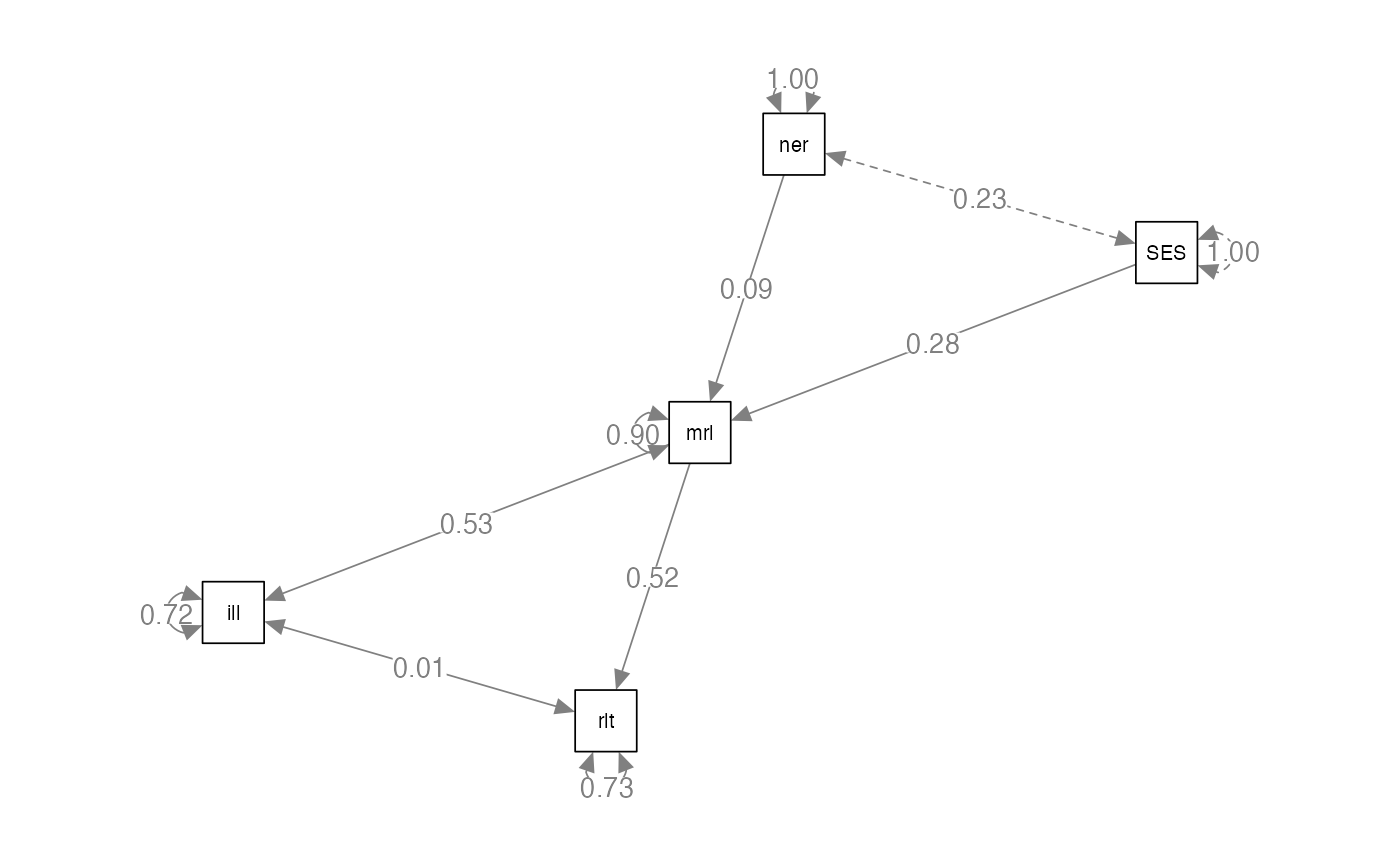

semPaths(compare.model2.fit, 
         whatLabels="par", 
         edge.label.cex = 1,
         layout="spring")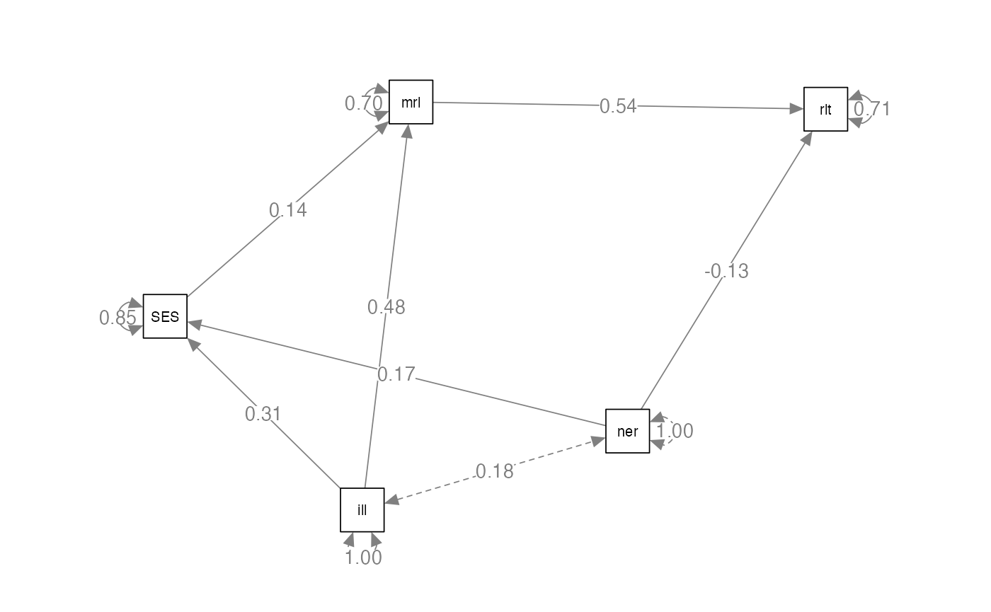

Compare the Models

anova(compare.model1.fit, compare.model2.fit)
#> 
#> Chi-Squared Difference Test
#> 
#>                    Df    AIC    BIC   Chisq Chisq diff   RMSEA Df diff
#> compare.model2.fit  3 3610.3 3647.6  3.2454                           
#> compare.model1.fit  4 3655.4 3688.6 40.3031     37.058 0.27728       1
#>                    Pr(>Chisq)    
#> compare.model2.fit               
#> compare.model1.fit  1.147e-09 ***
#> ---
#> Signif. codes:  0 '***' 0.001 '**' 0.01 '*' 0.05 '.' 0.1 ' ' 1
fitmeasures(compare.model1.fit, c("aic", "ecvi"))
#>      aic     ecvi 
#> 3655.377    0.120
fitmeasures(compare.model2.fit, c("aic", "ecvi"))
#>      aic     ecvi 
#> 3610.276    0.045

Summary

In this lecture you’ve learned:
- How to write basic lavaan model syntax
- How to analyze a path model
- How to summarize a path model
- How to create sem pictures
- Estimation and fit indices