Confirmatory Factor Analysis: Second Order
lecture_secondcfa.RmdSecond Order Latent Models
A second order model is one that is structured into an order or rank.
-
Two types we will consider:
- Higher-order: Describes when latent variables are structured so that latents influence other latents into levels.
- Bi-factor: Generally used to describe a CFA with two sets of latent variables (not hierarchical).
Second Order Models
-
The idea of a higher order model is:
- You have some latent variables that are measured by the observed variables.
- A portion of the variance in the latent variables can be explained by a second (set) of latent variables.
- Therefore, we are switching out the covariances between factors and using another latent to explain them.
Second Order Models
- When are these used?
- When there are multiple latent variables that covary with each other (and a lot).
- A second set of latents explains that covariance.
Higher Order Models
- The covariance of the first order is accounted for by the second order plus a specific factor.
- Specific factors are error that is not explained by the second order latents.
- The higher order is thought to indirectly influence the manifest variables through the first order.
Identification
-
Remember that each portion of the model has to be identified.
- The section with each latent variable has to be identified.
- The section with the latents has to be identified.
Identification
-
You can achieve identification in a couple of ways:
- Set some of the loadings in the upper portion of the model to be equal by giving them the same name.
- You can set the variance in the upper latent to be one.
- You can set some of the error variances of the latents in the lower portion to be equal.
Bi-Factor Models
Special type of model with two sets of latents, but they are not hierarchically structured.
-
Best used when:
- General factor that accounts for variance in the manifest variables.
- Domain specific areas that are thought to influence the manifest variables.
Bi-Factor Models
- One thing to note is that the latent variables are left uncorrelated in this type of model.
- This structure represents the domain specific part of the interpretation.
Model Differences
-
Differences between bi-factor and hierarchical:
- In hierarchical models, the second order influences the first order, while the two sets of latents in bi-factors are uncorrelated.
- What does that allow you to test differently?
Model Differences
-
Advantages:
- Allows you to see how the first order latent variables influence the manifest variables separately from the other latent variables.
- After accounting for the general latent variable, are the domain specific items still accounting for variance?
- You can compare models with and without the domain specific areas
Examples: WISC
- Going back to the WISC data, this time with more of the subscales that are available.
library(lavaan)
library(semPlot)

##import the data
wisc4.cov <- lav_matrix_lower2full(c(8.29,
                                    5.37,9.06,
                                    2.83,4.44,8.35,
                                    2.83,3.32,3.36,8.88,
                                    5.50,6.66,4.20,3.43,9.18,
                                    6.18,6.73,4.01,3.33,6.77,9.12,
                                    3.52,3.77,3.19,2.75,3.88,4.05,8.88,
                                    3.79,4.50,3.72,3.39,4.53,4.70,4.54,8.94,
                                    2.30,2.67,2.40,2.38,2.06,2.59,2.65,2.83,8.76,
                                    3.06,4.04,3.70,2.79,3.59,3.67,3.44,4.20,4.53,9.73))

wisc4.sd <- c(2.88,3.01,2.89,2.98,3.03,3.02,2.98,2.99,2.96,3.12)

names(wisc4.sd) <-
  colnames(wisc4.cov) <-
  rownames(wisc4.cov) <- c("Comprehension", "Information",
                         "Matrix.Reasoning", "Picture.Concepts",
                         "Similarities", "Vocabulary",  "Digit.Span",
                         "Letter.Number",  "Coding", "Symbol.Search")
Examples: WISC
- Let’s start with a first order model for the WISC.
- By starting with the measurement model, we can ensure the measurement section is identified and works correctly.
- You should also check out the correlations/covariances between factors to make sure that they are even related.
Examples: WISC Build the Model
##first order model
wisc4.fourFactor.model <- '
gc =~ Comprehension + Information +  Similarities + Vocabulary
gf =~ Matrix.Reasoning + Picture.Concepts
gsm =~  Digit.Span + Letter.Number
gs =~ Coding + Symbol.Search
'
Examples: WISC Analyze the Model
wisc4.fourFactor.fit <- cfa(model = wisc4.fourFactor.model,
                            sample.cov = wisc4.cov,
                            sample.nobs = 550)
Examples: WISC Summarize the Model
-
Logical solution:
- Positive variances
- SMCs + Correlations < 1
- No error messages
- SEs are not “huge”
-
Estimates:
- Do our questions load appropriately?
-
Model fit:
- What do the fit indices indicate?
- Can we improve model fit without overfitting?
summary(wisc4.fourFactor.fit,
        fit.measure = TRUE,
        standardized = TRUE,
        rsquare = TRUE)
#> lavaan 0.6-19 ended normally after 83 iterations
#>
#>   Estimator                                         ML
#>   Optimization method                           NLMINB
#>   Number of model parameters                        26
#>
#>   Number of observations                           550
#>
#> Model Test User Model:
#>
#>   Test statistic                                52.226
#>   Degrees of freedom                                29
#>   P-value (Chi-square)                           0.005
#>
#> Model Test Baseline Model:
#>
#>   Test statistic                              2554.487
#>   Degrees of freedom                                45
#>   P-value                                        0.000
#>
#> User Model versus Baseline Model:
#>
#>   Comparative Fit Index (CFI)                    0.991
#>   Tucker-Lewis Index (TLI)                       0.986
#>
#> Loglikelihood and Information Criteria:
#>
#>   Loglikelihood user model (H0)             -12562.889
#>   Loglikelihood unrestricted model (H1)     -12536.776
#>
#>   Akaike (AIC)                               25177.778
#>   Bayesian (BIC)                             25289.836
#>   Sample-size adjusted Bayesian (SABIC)      25207.301
#>
#> Root Mean Square Error of Approximation:
#>
#>   RMSEA                                          0.038
#>   90 Percent confidence interval - lower         0.021
#>   90 Percent confidence interval - upper         0.055
#>   P-value H_0: RMSEA <= 0.050                    0.876
#>   P-value H_0: RMSEA >= 0.080                    0.000
#>
#> Standardized Root Mean Square Residual:
#>
#>   SRMR                                           0.020
#>
#> Parameter Estimates:
#>
#>   Standard errors                             Standard
#>   Information                                 Expected
#>   Information saturated (h1) model          Structured
#>
#> Latent Variables:
#>                    Estimate  Std.Err  z-value  P(>|z|)   Std.lv  Std.all
#>   gc =~
#>     Comprehension     1.000                               2.193    0.762
#>     Information       1.160    0.056   20.802    0.000    2.544    0.846
#>     Similarities      1.166    0.056   20.772    0.000    2.558    0.845
#>     Vocabulary        1.218    0.056   21.860    0.000    2.670    0.885
#>   gf =~
#>     Matrix.Reasnng    1.000                               2.000    0.693
#>     Picture.Cncpts    0.839    0.078   10.775    0.000    1.677    0.563
#>   gsm =~
#>     Digit.Span        1.000                               1.967    0.661
#>     Letter.Number     1.172    0.086   13.560    0.000    2.304    0.771
#>   gs =~
#>     Coding            1.000                               1.779    0.601
#>     Symbol.Search     1.429    0.139   10.283    0.000    2.542    0.816
#>
#> Covariances:
#>                    Estimate  Std.Err  z-value  P(>|z|)   Std.lv  Std.all
#>   gc ~~
#>     gf                3.412    0.337   10.130    0.000    0.778    0.778
#>     gsm               3.302    0.336    9.826    0.000    0.766    0.766
#>     gs                2.180    0.290    7.511    0.000    0.559    0.559
#>   gf ~~
#>     gsm               3.245    0.352    9.220    0.000    0.825    0.825
#>     gs                2.507    0.329    7.608    0.000    0.705    0.705
#>   gsm ~~
#>     gs                2.474    0.324    7.627    0.000    0.707    0.707
#>
#> Variances:
#>                    Estimate  Std.Err  z-value  P(>|z|)   Std.lv  Std.all
#>    .Comprehension     3.467    0.240   14.452    0.000    3.467    0.419
#>    .Information       2.571    0.203   12.637    0.000    2.571    0.284
#>    .Similarities      2.622    0.207   12.672    0.000    2.622    0.286
#>    .Vocabulary        1.973    0.181   10.920    0.000    1.973    0.217
#>    .Matrix.Reasnng    4.336    0.424   10.224    0.000    4.336    0.520
#>    .Picture.Cncpts    6.051    0.434   13.944    0.000    6.051    0.683
#>    .Digit.Span        4.996    0.377   13.239    0.000    4.996    0.564
#>    .Letter.Number     3.614    0.381    9.499    0.000    3.614    0.405
#>    .Coding            5.581    0.428   13.053    0.000    5.581    0.638
#>    .Symbol.Search     3.249    0.573    5.668    0.000    3.249    0.335
#>     gc                4.807    0.468   10.270    0.000    1.000    1.000
#>     gf                3.999    0.544    7.353    0.000    1.000    1.000
#>     gsm               3.868    0.497    7.790    0.000    1.000    1.000
#>     gs                3.163    0.484    6.535    0.000    1.000    1.000
#>
#> R-Square:
#>                    Estimate
#>     Comprehension     0.581
#>     Information       0.716
#>     Similarities      0.714
#>     Vocabulary        0.783
#>     Matrix.Reasnng    0.480
#>     Picture.Cncpts    0.317
#>     Digit.Span        0.436
#>     Letter.Number     0.595
#>     Coding            0.362
#>     Symbol.Search     0.665
Examples: WISC Diagram the Model
semPaths(wisc4.fourFactor.fit,
         whatLabels="std",
         edge.label.cex = 1,
         edge.color = "black",
         what = "std",
         layout="tree")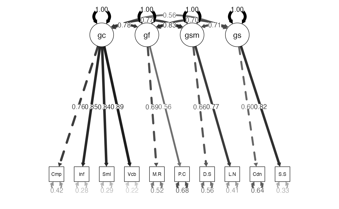
Examples: WISC Interpretation
- In the first order model, we find that the correlations are pretty high.
- That’s a good sign that maybe a second order model is appropriate.
- Or that the factors should be collapsed together, as they are not distinct.
Examples: Second-Order WISC
- Build the model:
wisc4.higherOrder.model <- '
gc =~ Comprehension + Information + Similarities + Vocabulary
gf =~ Matrix.Reasoning + Picture.Concepts
gsm =~  Digit.Span + Letter.Number
gs =~ Coding + Symbol.Search

g =~ gf + gc  + gsm + gs
'
Examples: Second-Order WISC
- Analyze the model:
wisc4.higherOrder.fit <- cfa(model = wisc4.higherOrder.model,
                             sample.cov = wisc4.cov,
                             sample.nobs = 550)
Examples: Second-Order WISC
-
Summarize the model:
- Note: the fit indices should not change.
- Let’s look at loadings, where the shift should have happened.
summary(wisc4.higherOrder.fit,
        fit.measure=TRUE,
        standardized=TRUE,
        rsquare = TRUE)
#> lavaan 0.6-19 ended normally after 67 iterations
#>
#>   Estimator                                         ML
#>   Optimization method                           NLMINB
#>   Number of model parameters                        24
#>
#>   Number of observations                           550
#>
#> Model Test User Model:
#>
#>   Test statistic                                58.180
#>   Degrees of freedom                                31
#>   P-value (Chi-square)                           0.002
#>
#> Model Test Baseline Model:
#>
#>   Test statistic                              2554.487
#>   Degrees of freedom                                45
#>   P-value                                        0.000
#>
#> User Model versus Baseline Model:
#>
#>   Comparative Fit Index (CFI)                    0.989
#>   Tucker-Lewis Index (TLI)                       0.984
#>
#> Loglikelihood and Information Criteria:
#>
#>   Loglikelihood user model (H0)             -12565.866
#>   Loglikelihood unrestricted model (H1)     -12536.776
#>
#>   Akaike (AIC)                               25179.732
#>   Bayesian (BIC)                             25283.170
#>   Sample-size adjusted Bayesian (SABIC)      25206.984
#>
#> Root Mean Square Error of Approximation:
#>
#>   RMSEA                                          0.040
#>   90 Percent confidence interval - lower         0.024
#>   90 Percent confidence interval - upper         0.056
#>   P-value H_0: RMSEA <= 0.050                    0.846
#>   P-value H_0: RMSEA >= 0.080                    0.000
#>
#> Standardized Root Mean Square Residual:
#>
#>   SRMR                                           0.023
#>
#> Parameter Estimates:
#>
#>   Standard errors                             Standard
#>   Information                                 Expected
#>   Information saturated (h1) model          Structured
#>
#> Latent Variables:
#>                    Estimate  Std.Err  z-value  P(>|z|)   Std.lv  Std.all
#>   gc =~
#>     Comprehension     1.000                               2.194    0.763
#>     Information       1.160    0.056   20.832    0.000    2.545    0.846
#>     Similarities      1.164    0.056   20.767    0.000    2.555    0.844
#>     Vocabulary        1.217    0.056   21.882    0.000    2.670    0.885
#>   gf =~
#>     Matrix.Reasnng    1.000                               1.991    0.690
#>     Picture.Cncpts    0.846    0.079   10.758    0.000    1.685    0.566
#>   gsm =~
#>     Digit.Span        1.000                               1.966    0.660
#>     Letter.Number     1.173    0.087   13.503    0.000    2.306    0.772
#>   gs =~
#>     Coding            1.000                               1.771    0.599
#>     Symbol.Search     1.441    0.142   10.149    0.000    2.553    0.819
#>   g =~
#>     gf                1.000                               0.930    0.930
#>     gc                0.968    0.079   12.241    0.000    0.817    0.817
#>     gsm               0.984    0.087   11.319    0.000    0.927    0.927
#>     gs                0.698    0.080    8.689    0.000    0.730    0.730
#>
#> Variances:
#>                    Estimate  Std.Err  z-value  P(>|z|)   Std.lv  Std.all
#>    .Comprehension     3.460    0.240   14.440    0.000    3.460    0.418
#>    .Information       2.565    0.203   12.614    0.000    2.565    0.284
#>    .Similarities      2.635    0.208   12.692    0.000    2.635    0.288
#>    .Vocabulary        1.973    0.181   10.906    0.000    1.973    0.217
#>    .Matrix.Reasnng    4.372    0.424   10.306    0.000    4.372    0.525
#>    .Picture.Cncpts    6.025    0.434   13.871    0.000    6.025    0.680
#>    .Digit.Span        5.000    0.378   13.219    0.000    5.000    0.564
#>    .Letter.Number     3.608    0.382    9.441    0.000    3.608    0.404
#>    .Coding            5.606    0.430   13.040    0.000    5.606    0.641
#>    .Symbol.Search     3.197    0.584    5.473    0.000    3.197    0.329
#>    .gc                1.599    0.226    7.082    0.000    0.332    0.332
#>    .gf                0.534    0.340    1.569    0.117    0.135    0.135
#>    .gsm               0.540    0.241    2.246    0.025    0.140    0.140
#>    .gs                1.467    0.262    5.590    0.000    0.468    0.468
#>     g                 3.429    0.452    7.591    0.000    1.000    1.000
#>
#> R-Square:
#>                    Estimate
#>     Comprehension     0.582
#>     Information       0.716
#>     Similarities      0.712
#>     Vocabulary        0.783
#>     Matrix.Reasnng    0.475
#>     Picture.Cncpts    0.320
#>     Digit.Span        0.436
#>     Letter.Number     0.596
#>     Coding            0.359
#>     Symbol.Search     0.671
#>     gc                0.668
#>     gf                0.865
#>     gsm               0.860
#>     gs                0.532
Examples: Second-Order WISC
semPaths(wisc4.higherOrder.fit,
         whatLabels="std",
         edge.label.cex = 1,
         edge.color = "black",
         what = "std",
         layout="tree")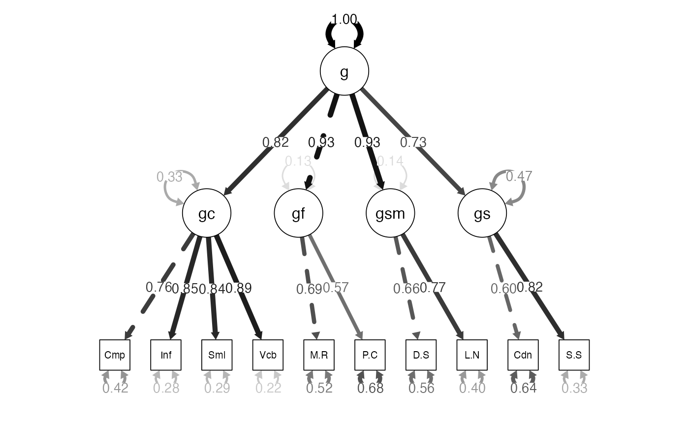
Examples: Bi-factor WISC
-
Build the model:
- In this particular model, because we have only two indicators, we have to set them equal for identification for a bifactor to run properly?
- Why not the second order model?
- After you define the measurement model, you would define a second latent that every variable is related to.
- Note: these are the variables not the latents like a hierarchical model.
wisc4.bifactor.model <- '
gc =~ Comprehension + Information +  Similarities + Vocabulary
gf =~ a*Matrix.Reasoning + a*Picture.Concepts
gsm =~  b*Digit.Span + b*Letter.Number
gs =~ c*Coding + c*Symbol.Search
g =~ Information + Comprehension + Matrix.Reasoning + Picture.Concepts + Similarities + Vocabulary +  Digit.Span + Letter.Number + Coding + Symbol.Search
'
Examples: Bi-factor WISC
-
Analyze the model:
- Last, we want to turn off the automatic exogenous only correlations,
which we do with the
orthogonal = TRUEmodel. - The argument is that all the correlations normally seen between the domain specific latents are due to the general factor.
- Last, we want to turn off the automatic exogenous only correlations,
which we do with the
wisc4.bifactor.fit <- cfa(model = wisc4.bifactor.model,
                          sample.cov = wisc4.cov,
                          sample.nobs = 550,
                          orthogonal = TRUE)
Examples: Bi-factor WISC
-
Summarize the model:
- Notice the covariances are zero.
- Notice the equal loading estimates for the variables set to the same.
summary(wisc4.bifactor.fit,
fit.measure = TRUE,
rsquare = TRUE,
standardized = TRUE)
#> lavaan 0.6-19 ended normally after 64 iterations
#>
#> Estimator ML
#> Optimization method NLMINB
#> Number of model parameters 27
#>
#> Number of observations 550
#>
#> Model Test User Model:
#>
#> Test statistic 50.833
#> Degrees of freedom 28
#> P-value (Chi-square) 0.005
#>
#> Model Test Baseline Model:
#>
#> Test statistic 2554.487
#> Degrees of freedom 45
#> P-value 0.000
#>
#> User Model versus Baseline Model:
#>
#> Comparative Fit Index (CFI) 0.991
#> Tucker-Lewis Index (TLI) 0.985
#>
#> Loglikelihood and Information Criteria:
#>
#> Loglikelihood user model (H0) -12562.192
#> Loglikelihood unrestricted model (H1) -12536.776
#>
#> Akaike (AIC) 25178.385
#> Bayesian (BIC) 25294.753
#> Sample-size adjusted Bayesian (SABIC) 25209.043
#>
#> Root Mean Square Error of Approximation:
#>
#> RMSEA 0.039
#> 90 Percent confidence interval - lower 0.021
#> 90 Percent confidence interval - upper 0.055
#> P-value H_0: RMSEA <= 0.050 0.864
#> P-value H_0: RMSEA >= 0.080 0.000
#>
#> Standardized Root Mean Square Residual:
#>
#> SRMR 0.022
#>
#> Parameter Estimates:
#>
#> Standard errors Standard
#> Information Expected
#> Information saturated (h1) model Structured
#>
#> Latent Variables:
#> Estimate Std.Err z-value P(>|z|) Std.lv Std.all
#> gc =~
#> Comprehnsn 1.000 1.426 0.496
#> Informatin 0.883 0.100 8.820 0.000 1.259 0.419
#> Similarits 0.965 0.106 9.134 0.000 1.375 0.454
#> Vocabulary 1.168 0.121 9.670 0.000 1.665 0.552
#> gf =~
#> Mtrx.Rsnng (a) 1.000 0.634 0.220
#> Pctr.Cncpt (a) 1.000 0.634 0.213
#> gsm =~
#> Digit.Span (b) 1.000 0.863 0.290
#> Lettr.Nmbr (b) 1.000 0.863 0.289
#> gs =~
#> Coding (c) 1.000 1.461 0.494
#> Symbl.Srch (c) 1.000 1.461 0.469
#> g =~
#> Informatin 1.000 2.191 0.728
#> Comprehnsn 0.780 0.051 15.388 0.000 1.709 0.594
#> Mtrx.Rsnng 0.859 0.066 13.107 0.000 1.883 0.652
#> Pctr.Cncpt 0.716 0.067 10.704 0.000 1.568 0.527
#> Similarits 0.972 0.051 18.880 0.000 2.130 0.704
#> Vocabulary 0.974 0.047 20.528 0.000 2.134 0.707
#> Digit.Span 0.818 0.068 11.971 0.000 1.792 0.602
#> Lettr.Nmbr 0.965 0.069 13.900 0.000 2.113 0.707
#> Coding 0.584 0.065 8.975 0.000 1.280 0.433
#> Symbl.Srch 0.851 0.069 12.262 0.000 1.865 0.598
#>
#> Covariances:
#> Estimate Std.Err z-value P(>|z|) Std.lv Std.all
#> gc ~~
#> gf 0.000 0.000 0.000
#> gsm 0.000 0.000 0.000
#> gs 0.000 0.000 0.000
#> g 0.000 0.000 0.000
#> gf ~~
#> gsm 0.000 0.000 0.000
#> gs 0.000 0.000 0.000
#> g 0.000 0.000 0.000
#> gsm ~~
#> gs 0.000 0.000 0.000
#> g 0.000 0.000 0.000
#> gs ~~
#> g 0.000 0.000 0.000
#>
#> Variances:
#> Estimate Std.Err z-value P(>|z|) Std.lv Std.all
#> .Comprehension 3.323 0.250 13.275 0.000 3.323 0.402
#> .Information 2.660 0.202 13.179 0.000 2.660 0.294
#> .Similarities 2.737 0.212 12.914 0.000 2.737 0.299
#> .Vocabulary 1.777 0.208 8.560 0.000 1.777 0.195
#> .Matrix.Reasnng 4.388 0.383 11.450 0.000 4.388 0.526
#> .Picture.Cncpts 6.004 0.444 13.534 0.000 6.004 0.677
#> .Digit.Span 4.908 0.381 12.890 0.000 4.908 0.554
#> .Letter.Number 3.713 0.345 10.751 0.000 3.713 0.416
#> .Coding 4.971 0.408 12.174 0.000 4.971 0.568
#> .Symbol.Search 4.100 0.391 10.489 0.000 4.100 0.422
#> gc 2.032 0.373 5.450 0.000 1.000 1.000
#> gf 0.402 0.280 1.437 0.151 1.000 1.000
#> gsm 0.745 0.282 2.640 0.008 1.000 1.000
#> gs 2.136 0.333 6.412 0.000 1.000 1.000
#> g 4.798 0.543 8.841 0.000 1.000 1.000
#>
#> R-Square:
#> Estimate
#> Comprehension 0.598
#> Information 0.706
#> Similarities 0.701
#> Vocabulary 0.805
#> Matrix.Reasnng 0.474
#> Picture.Cncpts 0.323
#> Digit.Span 0.446
#> Letter.Number 0.584
#> Coding 0.432
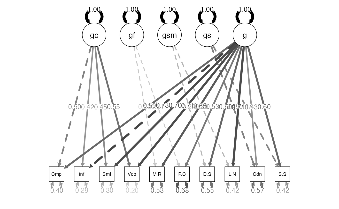
#> Symbol.Search 0.578Examples: Bi-factor WISC
- Diagram the model:
semPaths(wisc4.bifactor.fit,
         whatLabels="std",
         edge.label.cex = 1,
         edge.color = "black",
         what = "std",
         layout="tree")