Item Response Theory

Item Response Theory

• What do you do if you have dichotomous (or categorical) manifest variables?
  • Many agree that more than four response options can be treated as continuous without a loss in power or interpretation.
    
  • Do you treat these values as categorical?
• Do you assume the underlying latent variable is continuous?

Categorical Options

• There are two approaches that allow us to analyze data with categorical predictors:
  • Item Factor Analysis
    • More traditional factor analysis approach using ordered responses
    • You can talk about item loading, eliminate bad questions, etc.
    • In the lavaan framework, you update your cfa() to include the ordered argument
  • Item Response Theory

Item Response Theory

• Classical test theory is considered “true score theory”
  • Any differences in responses are differences in ability or underlying trait
  • CTT focuses on reliability and item correlation type analysis
  • Cannot separate the test and person characteristics
• IRT is considered more modern test theory focusing on the latent trait
  • Focuses on the item for where it measures a latent trait, discrimination, and guessing
  • Additionally, with more than two outcomes, we can examine ordering, response choice options, and more

Issues

• Unidimensionality: assumption is that there is one underlying trait or dimension you are measuring
  • You can run separate models for each dimension
  • There are multitrait options for IRT
• Local Independence
  • After you control for the latent variable, the items are uncorrelated

Item Response Theory

• A simple example of test versus person
  • 3 item questionnaire
  • Yes/no scaling
  • 8 response patterns
  • Four total scores (0, 1, 2, 3)

Item Response Theory

• Item characteristic curves (ICCs)
  • The log probability curve of theta and the probability of a correct response

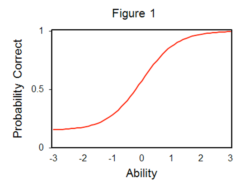
Item Response Theory

• Theta – ability or the underlying latent variable score
• b – Item location – where the probability of getting an item correct is 50/50
  • Also considered where the item performs best
  • Can be thought of as item difficulty

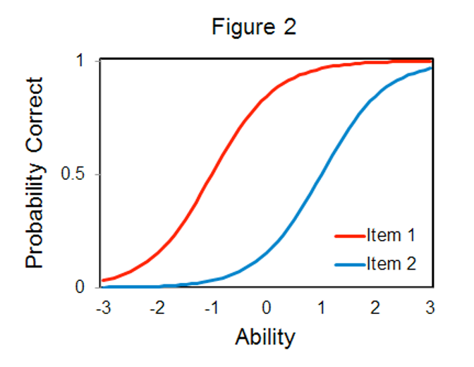
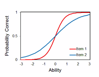
Item Response Theory

• a – item discrimination
  • Tells you how well an item measures the latent variable
  • Larger a values indicate better items

Item Response Theory

• c – guessing parameter
  • The lower level likelihood of getting the item correct

Item Response Theory

• 1 Parameter Logistic (1PL)
  • Also known as the Rasch Model
  • Only uses b
• 2 Parameter Logistic (2PL)
  • Uses b and a
• 3 Parameter Logistic (3PL)
  • Uses b, a, and c

Polytomous IRT

• A large portion of IRT focuses on dichotomous data (yes/no, correct/incorrect)
• Scoring is easier because you have “right” and “wrong” answers
• Separately, polytomous IRT focuses on data with multiple answers, with no “right” answer
  • Focus on ordering, meaning that low scores represent lower abilities, while high scores are higher abilities
  • Likert type scales

Polytomous IRT

• Couple of types of models:
  • Graded Response Model
  • Generalized Partial Credit Model
  • Partial Credit Model

Polytomous IRT

• A graded response model is simplest but can be hard to fit.
• Takes the number of categories – 1 and creates mini 2PLs for each of those boundary points (1-rest, 2-rest, 3-rest, etc.).
• You get probabilities of scoring at this level OR higher

Polytomous IRT

• The generalized partial credit and partial credit models account for the fact that you may not have each category used equally
• Therefore, you get the mini 2PLs for adjacent categories (1-2, 2-3, 3-4)
• If your categories are ordered (which you often want), these two estimations can be very similar.
• Another concern with the partial credit models is making sure that all categories have a point at which they are the most likely answer (thresholds)

Polytomous IRT

• Install the mirt() library to use the multidimensional IRT package.
• We are not covering multiple dimensional or multigroup IRT, but this package can do those models or polytomous estimation.

IRT Examples

• Let’s start with DIRT: Dichotomous IRT
• Dataset is the LSAT, which is scored as right or wrong

library(ltm)
#> Loading required package: MASS
#> Loading required package: msm
#> Loading required package: polycor
library(mirt)
#> Loading required package: stats4
#> Loading required package: lattice
#> 
#> Attaching package: 'mirt'
#> The following object is masked from 'package:ltm':
#> 
#>     Science
data(LSAT)
head(LSAT)
#>   Item 1 Item 2 Item 3 Item 4 Item 5
#> 1      0      0      0      0      0
#> 2      0      0      0      0      0
#> 3      0      0      0      0      0
#> 4      0      0      0      0      1
#> 5      0      0      0      0      1
#> 6      0      0      0      0      1

Two Parameter Logistic

# Data frame name ~ z1 for one latent variable
#irt.param to give it to you standardized
LSAT.model <- ltm(LSAT ~ z1,
                  IRT.param = TRUE)

2PL Output

• Difficulty = b = theta = ability
• Discrimination = a = how good the question is at figuring a person out.

coef(LSAT.model)
#>            Dffclt    Dscrmn
#> Item 1 -3.3597341 0.8253715
#> Item 2 -1.3696497 0.7229499
#> Item 3 -0.2798983 0.8904748
#> Item 4 -1.8659189 0.6885502
#> Item 5 -3.1235725 0.6574516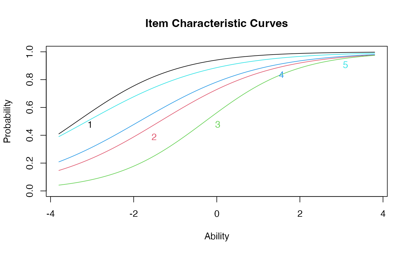

2PL Plots

plot(LSAT.model, type = "ICC") ## all items at once

2PL Plots

plot(LSAT.model, type = "IIC", items = 0) ## Test Information Function

2PL Other Options

factor.scores(LSAT.model)
#> 
#> Call:
#> ltm(formula = LSAT ~ z1, IRT.param = TRUE)
#> 
#> Scoring Method: Empirical Bayes
#> 
#> Factor-Scores for observed response patterns:
#>    Item 1 Item 2 Item 3 Item 4 Item 5 Obs     Exp     z1 se.z1
#> 1       0      0      0      0      0   3   2.277 -1.895 0.795
#> 2       0      0      0      0      1   6   5.861 -1.479 0.796
#> 3       0      0      0      1      0   2   2.596 -1.460 0.796
#> 4       0      0      0      1      1  11   8.942 -1.041 0.800
#> 5       0      0      1      0      0   1   0.696 -1.331 0.797
#> 6       0      0      1      0      1   1   2.614 -0.911 0.802
#> 7       0      0      1      1      0   3   1.179 -0.891 0.803
#> 8       0      0      1      1      1   4   5.955 -0.463 0.812
#> 9       0      1      0      0      0   1   1.840 -1.438 0.796
#> 10      0      1      0      0      1   8   6.431 -1.019 0.801
#> 11      0      1      0      1      1  16  13.577 -0.573 0.809
#> 12      0      1      1      0      1   3   4.370 -0.441 0.813
#> 13      0      1      1      1      0   2   2.000 -0.420 0.813
#> 14      0      1      1      1      1  15  13.920  0.023 0.828
#> 15      1      0      0      0      0  10   9.480 -1.373 0.797
#> 16      1      0      0      0      1  29  34.616 -0.953 0.802
#> 17      1      0      0      1      0  14  15.590 -0.933 0.802
#> 18      1      0      0      1      1  81  76.562 -0.506 0.811
#> 19      1      0      1      0      0   3   4.659 -0.803 0.804
#> 20      1      0      1      0      1  28  24.989 -0.373 0.815
#> 21      1      0      1      1      0  15  11.463 -0.352 0.815
#> 22      1      0      1      1      1  80  83.541  0.093 0.831
#> 23      1      1      0      0      0  16  11.254 -0.911 0.802
#> 24      1      1      0      0      1  56  56.105 -0.483 0.812
#> 25      1      1      0      1      0  21  25.646 -0.463 0.812
#> 26      1      1      0      1      1 173 173.310 -0.022 0.827
#> 27      1      1      1      0      0  11   8.445 -0.329 0.816
#> 28      1      1      1      0      1  61  62.520  0.117 0.832
#> 29      1      1      1      1      0  28  29.127  0.139 0.833
#> 30      1      1      1      1      1 298 296.693  0.606 0.855

Three Parameter Logistic

LSAT.model2 <- tpm(LSAT, #dataset
                   type = "latent.trait",
                   IRT.param = TRUE)
#> Warning in tpm(LSAT, type = "latent.trait", IRT.param = TRUE): Hessian matrix at convergence is not positive definite; unstable solution.

3PL Output

• Difficulty = b = theta = ability
• Discrimination = a = how good the question is at figuring a person out.
• Guessing = c = how easy the item is to guess

coef(LSAT.model2)
#>            Gussng     Dffclt     Dscrmn
#> Item 1 0.06389395 -3.3423509  0.8048523
#> Item 2 0.01567005 -1.5530954  0.6070241
#> Item 3 0.30088256  0.3301527 26.4150208
#> Item 4 0.06521055 -2.0342571  0.5700252
#> Item 5 0.02908352 -3.5826451  0.5523586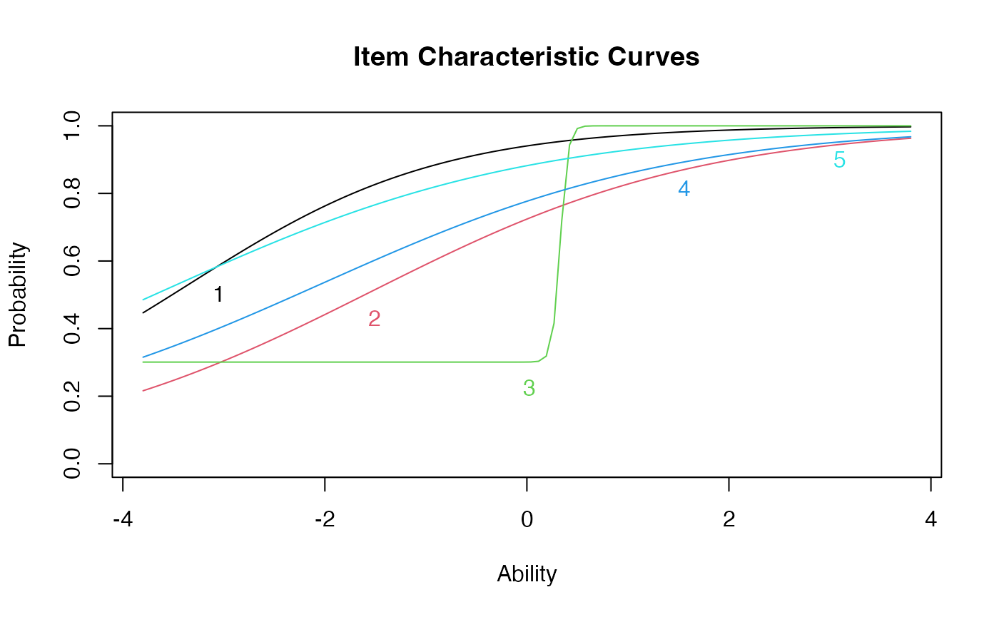

3PL Plots

plot(LSAT.model2, type = "ICC") ## all items at once

3PL Plots

plot(LSAT.model2, type = "IIC", items = 0) ## Test Information Function

3PL Other Options

factor.scores(LSAT.model2)
#> 
#> Call:
#> tpm(data = LSAT, type = "latent.trait", IRT.param = TRUE)
#> 
#> Scoring Method: Empirical Bayes
#> 
#> Factor-Scores for observed response patterns:
#>    Item 1 Item 2 Item 3 Item 4 Item 5 Obs     Exp     z1 se.z1
#> 1       0      0      0      0      0   3   1.538 -1.659 0.865
#> 2       0      0      0      0      1   6   5.113 -1.245 0.876
#> 3       0      0      0      1      0   2   2.375 -1.245 0.879
#> 4       0      0      0      1      1  11   9.552 -0.815 0.891
#> 5       0      0      1      0      0   1   0.686 -1.659 0.865
#> 6       0      0      1      0      1   1   2.472 -1.245 0.876
#> 7       0      0      1      1      0   3   1.149 -1.245 0.879
#> 8       0      0      1      1      1   4   5.597 -0.815 0.891
#> 9       0      1      0      0      0   1   1.678 -1.205 0.878
#> 10      0      1      0      0      1   8   6.870 -0.777 0.890
#> 11      0      1      0      1      1  16  15.339 -0.330 0.906
#> 12      0      1      1      0      1   3   4.118 -0.777 0.890
#> 13      0      1      1      1      0   2   1.917 -0.774 0.893
#> 14      0      1      1      1      1  15  13.227 -0.330 0.906
#> 15      1      0      0      0      0  10   7.980 -1.053 0.883
#> 16      1      0      0      0      1  29  34.733 -0.619 0.895
#> 17      1      0      0      1      0  14  16.116 -0.616 0.898
#> 18      1      0      0      1      1  81  81.511 -0.166 0.910
#> 19      1      0      1      0      0   3   4.134 -1.053 0.883
#> 20      1      0      1      0      1  28  23.238 -0.619 0.895
#> 21      1      0      1      1      0  15  10.828 -0.616 0.898
#> 22      1      0      1      1      1  80  83.177 -0.166 0.912
#> 23      1      1      0      0      0  16  11.668 -0.577 0.897
#> 24      1      1      0      0      1  56  59.731 -0.129 0.908
#> 25      1      1      0      1      0  21  27.722 -0.122 0.910
#> 26      1      1      0      1      1 173 158.900  0.150 0.376
#> 27      1      1      1      0      0  11   8.068 -0.577 0.897
#> 28      1      1      1      0      1  61  63.489 -0.128 0.913
#> 29      1      1      1      1      0  28  29.695 -0.122 0.916
#> 30      1      1      1      1      1 298 303.369  0.503 0.407

Compare Models

anova(LSAT.model, LSAT.model2)
#> Warning in anova.ltm(LSAT.model, LSAT.model2): either the two models are not nested or the model represented by 'object2' fell on a local maxima.
#> 
#>  Likelihood Ratio Table
#>                 AIC     BIC  log.Lik   LRT df p.value
#> LSAT.model  4953.31 5002.38 -2466.65                 
#> LSAT.model2 4967.02 5040.64 -2468.51 -3.71  5       1

Polytomous IRT

• Dataset includes the Meaning in Life Questionnaire

library(rio)
poly.data <- import("data/lecture_irt.csv")
poly.data <- na.omit(poly.data)

#reverse code
poly.data$Q99_9 = 8 - poly.data$Q99_9

#separate factors
poly.data1 = poly.data[ , c(1, 4, 5, 6, 9)]
poly.data2 = poly.data[ , c(2, 3, 7, 8, 10)]

Graded Partial Credit Model

gpcm.model1 <- mirt(data = poly.data1, #data
                    model = 1, #number of factors
                    itemtype = "gpcm") #poly model type
#> Iteration: 1, Log-Lik: -11632.167, Max-Change: 4.82538Iteration: 2, Log-Lik: -10643.196, Max-Change: 2.80519Iteration: 3, Log-Lik: -10466.648, Max-Change: 1.46456Iteration: 4, Log-Lik: -10407.465, Max-Change: 1.07570Iteration: 5, Log-Lik: -10391.165, Max-Change: 0.70497Iteration: 6, Log-Lik: -10380.881, Max-Change: 0.46272Iteration: 7, Log-Lik: -10377.111, Max-Change: 0.31365Iteration: 8, Log-Lik: -10374.263, Max-Change: 0.21356Iteration: 9, Log-Lik: -10372.203, Max-Change: 0.38073Iteration: 10, Log-Lik: -10369.957, Max-Change: 0.15524Iteration: 11, Log-Lik: -10368.478, Max-Change: 0.22565Iteration: 12, Log-Lik: -10367.024, Max-Change: 0.16375Iteration: 13, Log-Lik: -10364.773, Max-Change: 0.09306Iteration: 14, Log-Lik: -10363.888, Max-Change: 0.14681Iteration: 15, Log-Lik: -10363.042, Max-Change: 0.13197Iteration: 16, Log-Lik: -10360.346, Max-Change: 0.12133Iteration: 17, Log-Lik: -10359.333, Max-Change: 0.03727Iteration: 18, Log-Lik: -10359.002, Max-Change: 0.04397Iteration: 19, Log-Lik: -10358.801, Max-Change: 0.04719Iteration: 20, Log-Lik: -10358.591, Max-Change: 0.05133Iteration: 21, Log-Lik: -10358.410, Max-Change: 0.02077Iteration: 22, Log-Lik: -10358.337, Max-Change: 0.04891Iteration: 23, Log-Lik: -10358.184, Max-Change: 0.03701Iteration: 24, Log-Lik: -10358.050, Max-Change: 0.01716Iteration: 25, Log-Lik: -10358.005, Max-Change: 0.03666Iteration: 26, Log-Lik: -10357.894, Max-Change: 0.03487Iteration: 27, Log-Lik: -10357.797, Max-Change: 0.01621Iteration: 28, Log-Lik: -10357.767, Max-Change: 0.01415Iteration: 29, Log-Lik: -10357.694, Max-Change: 0.04601Iteration: 30, Log-Lik: -10357.617, Max-Change: 0.03283Iteration: 31, Log-Lik: -10357.524, Max-Change: 0.01379Iteration: 32, Log-Lik: -10357.474, Max-Change: 0.03921Iteration: 33, Log-Lik: -10357.424, Max-Change: 0.00916Iteration: 34, Log-Lik: -10357.416, Max-Change: 0.01006Iteration: 35, Log-Lik: -10357.380, Max-Change: 0.02822Iteration: 36, Log-Lik: -10357.343, Max-Change: 0.00895Iteration: 37, Log-Lik: -10357.337, Max-Change: 0.00870Iteration: 38, Log-Lik: -10357.310, Max-Change: 0.00980Iteration: 39, Log-Lik: -10357.287, Max-Change: 0.03201Iteration: 40, Log-Lik: -10357.257, Max-Change: 0.00613Iteration: 41, Log-Lik: -10357.241, Max-Change: 0.00621Iteration: 42, Log-Lik: -10357.226, Max-Change: 0.00628Iteration: 43, Log-Lik: -10357.203, Max-Change: 0.00560Iteration: 44, Log-Lik: -10357.190, Max-Change: 0.00178Iteration: 45, Log-Lik: -10357.186, Max-Change: 0.00399Iteration: 46, Log-Lik: -10357.179, Max-Change: 0.00227Iteration: 47, Log-Lik: -10357.176, Max-Change: 0.03798Iteration: 48, Log-Lik: -10357.155, Max-Change: 0.00415Iteration: 49, Log-Lik: -10357.155, Max-Change: 0.00413Iteration: 50, Log-Lik: -10357.148, Max-Change: 0.00366Iteration: 51, Log-Lik: -10357.144, Max-Change: 0.00372Iteration: 52, Log-Lik: -10357.131, Max-Change: 0.04537Iteration: 53, Log-Lik: -10357.110, Max-Change: 0.00132Iteration: 54, Log-Lik: -10357.109, Max-Change: 0.00345Iteration: 55, Log-Lik: -10357.106, Max-Change: 0.00159Iteration: 56, Log-Lik: -10357.105, Max-Change: 0.00040Iteration: 57, Log-Lik: -10357.104, Max-Change: 0.00058Iteration: 58, Log-Lik: -10357.104, Max-Change: 0.00021Iteration: 59, Log-Lik: -10357.104, Max-Change: 0.00047Iteration: 60, Log-Lik: -10357.104, Max-Change: 0.00016Iteration: 61, Log-Lik: -10357.104, Max-Change: 0.00013Iteration: 62, Log-Lik: -10357.104, Max-Change: 0.00025Iteration: 63, Log-Lik: -10357.104, Max-Change: 0.00012Iteration: 64, Log-Lik: -10357.104, Max-Change: 0.00010

GPCM Output

• Can also get factor loadings here, with standardized coefficients to help us determine if they relate to their latent trait

summary(gpcm.model1) ##standardized coefficients 
#>          F1    h2
#> Q99_1 0.964 0.929
#> Q99_4 0.984 0.968
#> Q99_5 0.976 0.953
#> Q99_6 0.977 0.955
#> Q99_9 0.720 0.519
#> 
#> SS loadings:  4.324 
#> Proportion Var:  0.865 
#> 
#> Factor correlations: 
#> 
#>    F1
#> F1  1

GPCM Output

coef(gpcm.model1, IRTpars = T) ##coefficients
#> $Q99_1
#>         a     b1     b2     b3     b4    b5    b6
#> par 1.927 -1.905 -1.344 -1.107 -0.607 0.225 1.236
#> 
#> $Q99_4
#>         a     b1    b2     b3     b4    b5    b6
#> par 2.941 -1.952 -1.67 -1.082 -0.592 0.121 0.972
#> 
#> $Q99_5
#>         a     b1     b2     b3     b4     b5    b6
#> par 2.395 -2.052 -1.601 -1.255 -0.825 -0.093 0.979
#> 
#> $Q99_6
#>         a     b1    b2     b3     b4    b5    b6
#> par 2.448 -2.014 -1.43 -1.168 -0.531 0.118 1.085
#> 
#> $Q99_9
#>         a     b1     b2     b3     b4     b5     b6
#> par 0.553 -1.671 -2.488 -1.202 -0.113 -1.115 -0.296
#> 
#> $GroupPars
#>     MEAN_1 COV_11
#> par      0      1

head(fscores(gpcm.model1)) ##factor scores
#>              F1
#> [1,] -0.6805579
#> [2,] -2.7481783
#> [3,] -1.2486173
#> [4,] -1.4226850
#> [5,] -2.7481783
#> [6,] -2.7481783

GPCM Plots

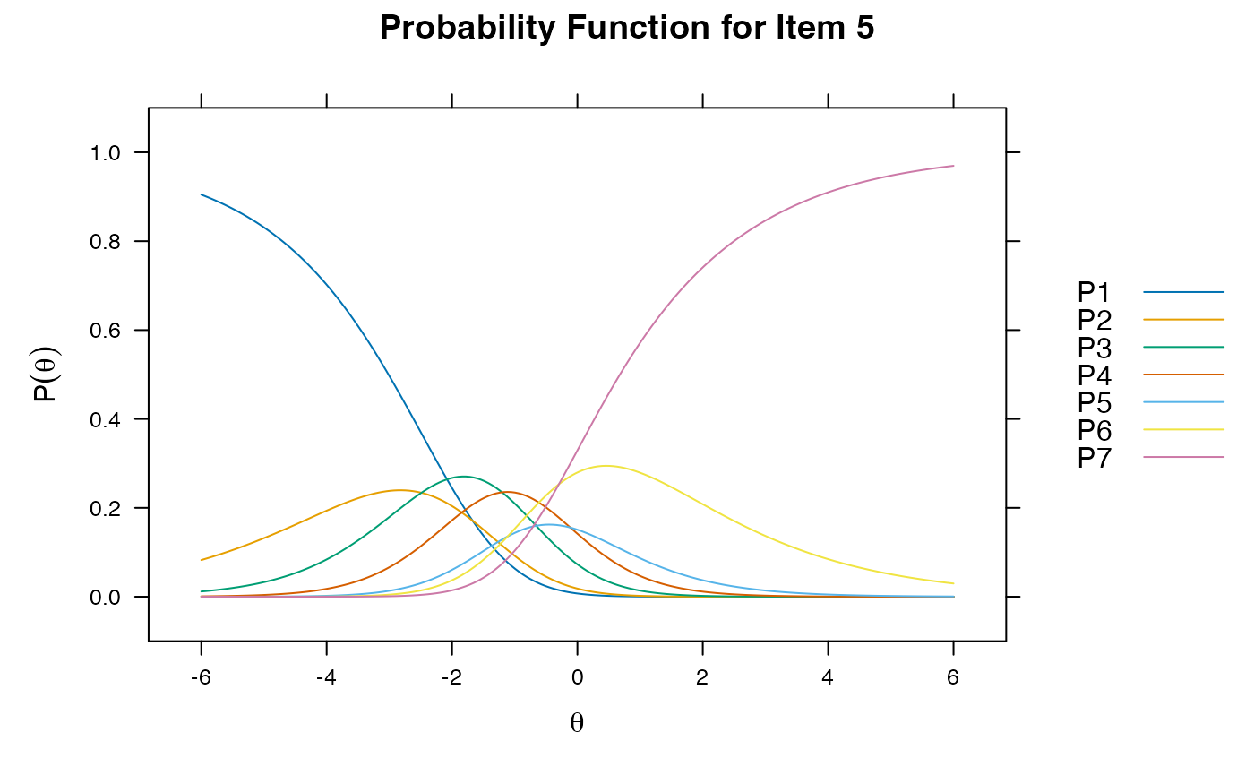
plot(gpcm.model1, type = "trace") ##curves for all items at once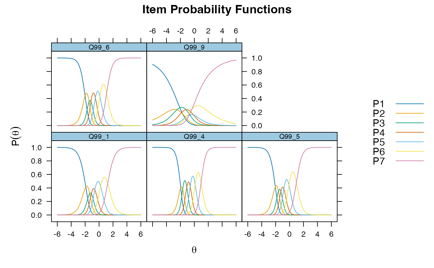

itemplot(gpcm.model1, 5, type = "trace")

GPCM Plots

itemplot(gpcm.model1, 4, type = "info") ##IIC for each item

plot(gpcm.model1, type = "info") ##test information curve

GPCM Plots

plot(gpcm.model1) ##expected score curve

Summary

• In this lecture you’ve learned:

  • Item response theory compared to classical test theory
  • How to run a dichotomous or traditional IRT with 2PL and 3PL
  • How to run a polytomous IRT using graded partial credit model
  • How to compare models and interpret their output