Multi-Group Confirmatory Factor Analysis
lecture_mgcfa.RmdMultigroup Models
- Let’s start with some terminology specific to multigroup models: invariance = equivalence
- Under different conditions, do the measurements yield the same measurement of attributes?
- Generally, we’ve seen that latent variable models are estimating the data based on the covariances. For these models, we will also add the mean structure.
- While you can test many groups in these models, you will want to generally compare two at a time.
Mean Structure
- Mean structure represents the intercept of our manifest variables
- In regression, remember that the Y-intercept is the mean of Y (given
X = 0 or no X variables)
- That’s your best guess for what someone is going to score on that item without any other X information
- Same idea in a latent variable model - it’s the starting value for that manifest variable.
Latent Means
- Latent means are the estimated score on the latent variable for participants.
- It’s a weighted score of each item’s original value with their path coefficient, and all items are averaged together.
- We can use
lavPredict()to calculate these for us.
Multigroup Questions
- Do items act the same across groups?
- Is the factor structure the same across groups?
- Are the paths equal across groups?
- Are the latent means equal across groups?
How to MG
- First, test the model as a regular CFA with everyone in the dataset
- This model will tell you if you have problems with your CFA
- This model is the least restrictive
- Do not use grouping variables
How to MG
- Second, test each group separately with the same CFA structure to determine that each individual group fits ok.
- Fit indices often decrease slightly here, because sample size is smaller (which usually has a bit more error variance).
- Mainly, you are looking for models that completely break down
- You could have a poor fitting CFA overall and use this step to see if that’s because one group just does not fit.
How to MG
- The next steps will be to nest the two models together.
- Nesting is like stacking the models together (like pancakes).
- For the nested model steps, most people use Brown’s terminology and procedure.
How to MG
- All the possible paths:
- The whole model (the picture)
- Loadings (regression weights)
- Intercepts (y-intercept for each item)
- Error variances (variance)
- Factor variances (variances for the latents)
- Factor covariances (correlation)
- Factor means (latent means)
Equal Form / Configural Invariance
- In this model, you put the two groups together into the same model.
- You do not force any of the paths to be the same, but you are forcing the model picture to be the same.
- You are testing if both groups show the same factor structure (configuration).
Metric Invariance
- In this model, you are forcing all the factor loadings (regression weights) to be exactly the same.
- This step will tell you if the groups have the same weights for each question – or if some questions have different signs or strengths.
Scalar Invariance
- In this model, you are forcing the intercepts of the items to be the same.
- This step will tell you if items have the same starting point – remember that the y-intercept is the mean of the item.
- If a MG model is going to indicate non-invariance – this step is often the one that breaks.
Strict Factorial Invariance
- In this model, you are forcing the error variances for each item to be the same.
- This step will tell you if the variance (the spread) of the item is
the same for each group.
- If you get differences, that indicates one group has a larger range of answers than another, which indicates they are more heterogeneous.
Other Steps
- Most of the previous steps are on the manifest/measured variables only.
- Generally, we focus on those because they indicate performance of the scale.
- Population Heterogeneity:
- Equal factor variances: Testing if latents have the same set of variance – means that the overall score has the same spread
- Equal factor covariances: Testing if the correlations between factors is the same for each group
- Equal latent means: Testing if the overall latent means are equal for each group
How to Judge
- How can I tell if steps are invariant?
- You will expect fit to get worse as you go because you are being more and more restrictive.
- While we can use change in , most suggest a change in CFI > .01 to be a difference in fit.
Model Breakdown
- What do I do if steps are NOT invariant?
- Partial invariance – when strict invariance cannot be met, you can test for partial invariance
- Partial invariance occurs when most of the items are invariant but a couple.
- You have to meet the invariance criteria, so you trying to bring your bad model “up” to the invariant level
- You want to do as few of items as possible
Partial Invariance
- So, how do I test partial invariance?
- We can use modification indices to see which paths are the most problematic.
- You will change ONE item at a time.
- Slowly add items to bring CFI up to an acceptable change level (i.e. .01 or less change from the previous model).
Test Latent Means
- After saying the measured variables are partially to fully
invariant, sometimes people also calculate latent means and use
t-tests to determine if they are different by groups.
- Instead of doing all the population heterogeneity steps.
- At the minimum, it is useful to know how to calculate a weighted score for each participant.
- We normally use EFA/CFA to show that each question has a nice loading and the questions load together
- And then we use subtotals or averages to create an overall score for
each latent
- This procedure totally ignores the fact that loadings are often different.
- Why lose that information?
Let’s get started!
- Equality constraints
- We’ve talked before about setting paths equal to each other by
calling them the same parameter name
cheese =~ a\*feta + a\*swiss- So feta and swiss will be estimated at the same value.
- The entire purpose of a multigroup model is to build equality constraints
- A few packages used to do this … but have become more trouble than
they are worth, so let’s look at how to do these steps with just
lavaan.
An Example
- Using the RS-14 scale: a one-factor measure of resiliency
library(lavaan)
library(rio)
res.data <- import("data/assignment_mgcfa.csv")

head(res.data)
#>   Sex Ethnicity RS1 RS2 RS3 RS4 RS5 RS6 RS7 RS8 RS9 RS10 RS11 RS12 RS13 RS14
#> 1   2         0   4   4   4   4   4   4   4   4   4    4    4    4    4    4
#> 2   1         0   5   2   6   4   4   5   4   5   5    4    4    6    4    4
#> 3   2         0   7   7   7   7   2   7   7   4   3    7    7    5    7    5
#> 4   2         0   7   6   6   7   7   7   7   7   7    7    7    6    7    7
#> 5   1         0   2   2   2   2   2   2   2   2   2    2    2    2    2    2
#> 6 2 0 4 5 5 7 5 7 5 7 5 4 5 6 6 5Start with Overall CFA
- NEW:
meanstructure = TRUE - Gives you the intercepts and means in the model.
- You want to turn that one at the beginning, and you are first examining models with means, so you can tell if you have bad parameters at the start.
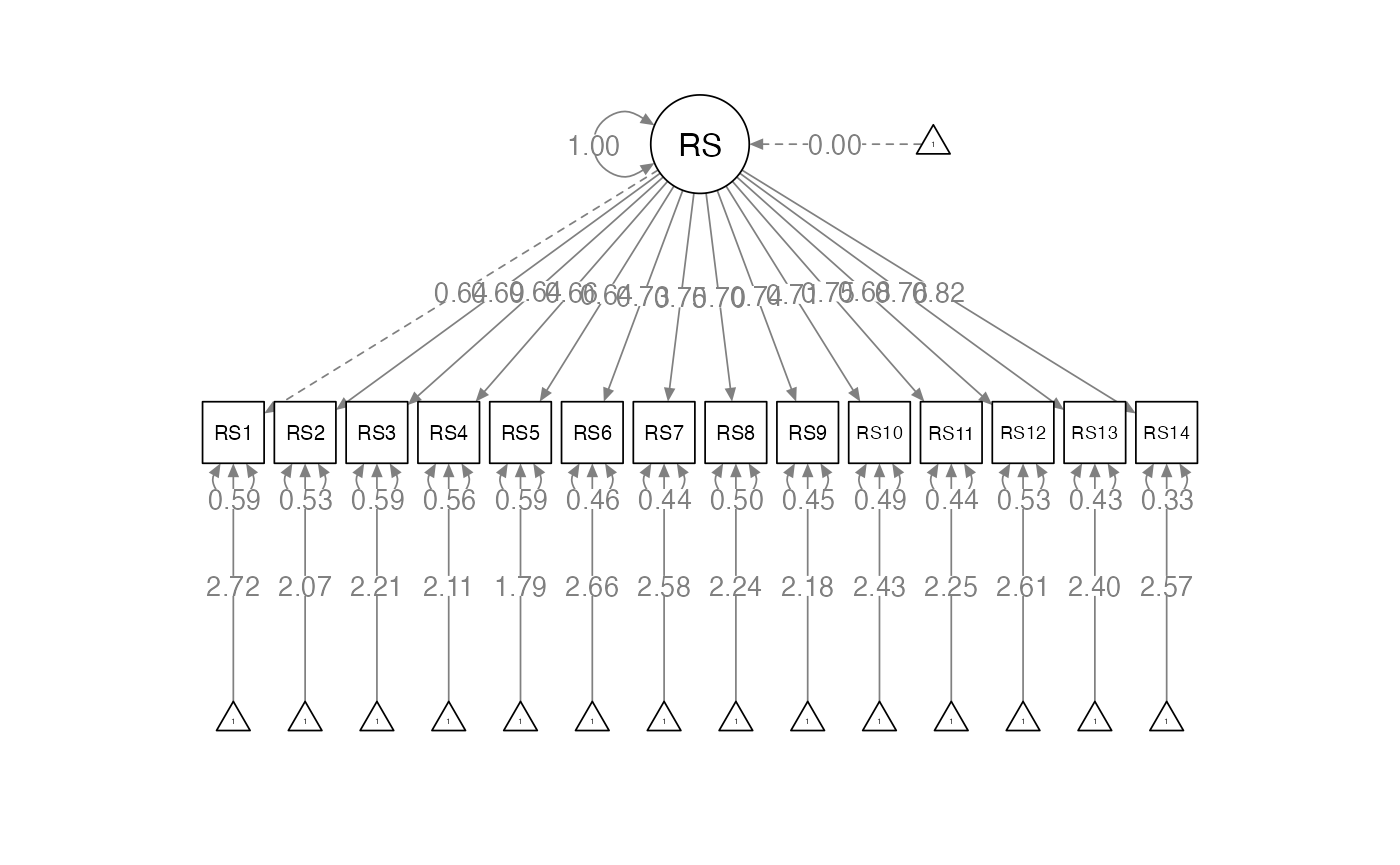
Start with Overall CFA
overall.model <- '
RS =~ RS1 + RS2 + RS3 + RS4 + RS5 + RS6 + RS7 + RS8 + RS9 + RS10 + RS11 + RS12 + RS13 + RS14
'

overall.fit <- cfa(model = overall.model,
                   data = res.data,
                   meanstructure = TRUE) ##this is important
Examine Overall Fit
summary(overall.fit,
        standardized = TRUE,
        rsquare = TRUE,
        fit.measure = TRUE)
#> lavaan 0.6-19 ended normally after 26 iterations
#>
#>   Estimator                                         ML
#>   Optimization method                           NLMINB
#>   Number of model parameters                        42
#>
#>   Number of observations                           510
#>
#> Model Test User Model:
#>
#>   Test statistic                               368.984
#>   Degrees of freedom                                77
#>   P-value (Chi-square)                           0.000
#>
#> Model Test Baseline Model:
#>
#>   Test statistic                              4064.761
#>   Degrees of freedom                                91
#>   P-value                                        0.000
#>
#> User Model versus Baseline Model:
#>
#>   Comparative Fit Index (CFI)                    0.927
#>   Tucker-Lewis Index (TLI)                       0.913
#>
#> Loglikelihood and Information Criteria:
#>
#>   Loglikelihood user model (H0)             -13050.226
#>   Loglikelihood unrestricted model (H1)     -12865.734
#>
#>   Akaike (AIC)                               26184.452
#>   Bayesian (BIC)                             26362.297
#>   Sample-size adjusted Bayesian (SABIC)      26228.983
#>
#> Root Mean Square Error of Approximation:
#>
#>   RMSEA                                          0.086
#>   90 Percent confidence interval - lower         0.078
#>   90 Percent confidence interval - upper         0.095
#>   P-value H_0: RMSEA <= 0.050                    0.000
#>   P-value H_0: RMSEA >= 0.080                    0.882
#>
#> Standardized Root Mean Square Residual:
#>
#>   SRMR                                           0.041
#>
#> Parameter Estimates:
#>
#>   Standard errors                             Standard
#>   Information                                 Expected
#>   Information saturated (h1) model          Structured
#>
#> Latent Variables:
#>                    Estimate  Std.Err  z-value  P(>|z|)   Std.lv  Std.all
#>   RS =~
#>     RS1               1.000                               1.135    0.637
#>     RS2               1.230    0.091   13.529    0.000    1.397    0.685
#>     RS3               1.065    0.083   12.806    0.000    1.209    0.641
#>     RS4               1.231    0.094   13.150    0.000    1.398    0.662
#>     RS5               1.203    0.094   12.846    0.000    1.366    0.644
#>     RS6               1.218    0.085   14.258    0.000    1.383    0.732
#>     RS7               1.264    0.087   14.554    0.000    1.435    0.751
#>     RS8               1.207    0.087   13.836    0.000    1.371    0.705
#>     RS9               1.271    0.088   14.461    0.000    1.444    0.745
#>     RS10              1.193    0.086   13.946    0.000    1.355    0.712
#>     RS11              1.318    0.091   14.526    0.000    1.496    0.749
#>     RS12              1.156    0.086   13.494    0.000    1.312    0.683
#>     RS13              1.357    0.093   14.634    0.000    1.541    0.756
#>     RS14              1.335    0.086   15.587    0.000    1.515    0.821
#>
#> Intercepts:
#>                    Estimate  Std.Err  z-value  P(>|z|)   Std.lv  Std.all
#>    .RS1               4.849    0.079   61.416    0.000    4.849    2.720
#>    .RS2               4.218    0.090   46.752    0.000    4.218    2.070
#>    .RS3               4.163    0.084   49.853    0.000    4.163    2.208
#>    .RS4               4.451    0.094   47.600    0.000    4.451    2.108
#>    .RS5               3.808    0.094   40.536    0.000    3.808    1.795
#>    .RS6               5.037    0.084   60.180    0.000    5.037    2.665
#>    .RS7               4.937    0.085   58.353    0.000    4.937    2.584
#>    .RS8               4.351    0.086   50.508    0.000    4.351    2.237
#>    .RS9               4.233    0.086   49.333    0.000    4.233    2.185
#>    .RS10              4.622    0.084   54.829    0.000    4.622    2.428
#>    .RS11              4.486    0.088   50.739    0.000    4.486    2.247
#>    .RS12              5.006    0.085   58.865    0.000    5.006    2.607
#>    .RS13              4.894    0.090   54.257    0.000    4.894    2.403
#>    .RS14              4.749    0.082   58.132    0.000    4.749    2.574
#>
#> Variances:
#>                    Estimate  Std.Err  z-value  P(>|z|)   Std.lv  Std.all
#>    .RS1               1.890    0.124   15.242    0.000    1.890    0.594
#>    .RS2               2.200    0.146   15.025    0.000    2.200    0.530
#>    .RS3               2.094    0.138   15.225    0.000    2.094    0.589
#>    .RS4               2.504    0.165   15.137    0.000    2.504    0.562
#>    .RS5               2.636    0.173   15.215    0.000    2.636    0.586
#>    .RS6               1.660    0.113   14.740    0.000    1.660    0.465
#>    .RS7               1.591    0.109   14.588    0.000    1.591    0.436
#>    .RS8               1.905    0.128   14.917    0.000    1.905    0.503
#>    .RS9               1.671    0.114   14.639    0.000    1.671    0.445
#>    .RS10              1.788    0.120   14.875    0.000    1.788    0.493
#>    .RS11              1.749    0.120   14.604    0.000    1.749    0.439
#>    .RS12              1.966    0.131   15.036    0.000    1.966    0.533
#>    .RS13              1.776    0.122   14.543    0.000    1.776    0.428
#>    .RS14              1.107    0.081   13.753    0.000    1.107    0.325
#>     RS                1.289    0.164    7.847    0.000    1.000    1.000
#>
#> R-Square:
#>                    Estimate
#>     RS1               0.406
#>     RS2               0.470
#>     RS3               0.411
#>     RS4               0.438
#>     RS5               0.414
#>     RS6               0.535
#>     RS7               0.564
#>     RS8               0.497
#>     RS9               0.555
#>     RS10              0.507
#>     RS11              0.561
#>     RS12              0.467
#>     RS13              0.572
#>     RS14              0.675
Make a table of fit indices
library(knitr)
table_fit <- matrix(NA, nrow = 9, ncol = 6)
colnames(table_fit) = c("Model", "X2", "df", "CFI", "RMSEA", "SRMR")
table_fit[1, ] <- c("Overall Model", round(fitmeasures(overall.fit,
                                                 c("chisq", "df", "cfi",
                                                   "rmsea", "srmr")),3))
kable(table_fit)| Model | X2 | df | CFI | RMSEA | SRMR |
|---|---|---|---|---|---|
| Overall Model | 368.984 | 77 | 0.927 | 0.086 | 0.041 |
| NA | NA | NA | NA | NA | NA |
| NA | NA | NA | NA | NA | NA |
| NA | NA | NA | NA | NA | NA |
| NA | NA | NA | NA | NA | NA |
| NA | NA | NA | NA | NA | NA |
| NA | NA | NA | NA | NA | NA |
| NA | NA | NA | NA | NA | NA |
| NA | NA | NA | NA | NA | NA |
Men Overall Summary
men.fit <- cfa(model = overall.model,
               data = res.data[res.data$Sex == "Men" , ],
               meanstructure = TRUE)
summary(men.fit,
        standardized = TRUE,
        rsquare = TRUE,
        fit.measure = TRUE)
#> lavaan 0.6-19 ended normally after 25 iterations
#>
#>   Estimator                                         ML
#>   Optimization method                           NLMINB
#>   Number of model parameters                        42
#>
#>   Number of observations                           244
#>
#> Model Test User Model:
#>
#>   Test statistic                               271.457
#>   Degrees of freedom                                77
#>   P-value (Chi-square)                           0.000
#>
#> Model Test Baseline Model:
#>
#>   Test statistic                              2515.572
#>   Degrees of freedom                                91
#>   P-value                                        0.000
#>
#> User Model versus Baseline Model:
#>
#>   Comparative Fit Index (CFI)                    0.920
#>   Tucker-Lewis Index (TLI)                       0.905
#>
#> Loglikelihood and Information Criteria:
#>
#>   Loglikelihood user model (H0)              -6043.672
#>   Loglikelihood unrestricted model (H1)      -5907.944
#>
#>   Akaike (AIC)                               12171.345
#>   Bayesian (BIC)                             12318.226
#>   Sample-size adjusted Bayesian (SABIC)      12185.091
#>
#> Root Mean Square Error of Approximation:
#>
#>   RMSEA                                          0.102
#>   90 Percent confidence interval - lower         0.089
#>   90 Percent confidence interval - upper         0.115
#>   P-value H_0: RMSEA <= 0.050                    0.000
#>   P-value H_0: RMSEA >= 0.080                    0.997
#>
#> Standardized Root Mean Square Residual:
#>
#>   SRMR                                           0.041
#>
#> Parameter Estimates:
#>
#>   Standard errors                             Standard
#>   Information                                 Expected
#>   Information saturated (h1) model          Structured
#>
#> Latent Variables:
#>                    Estimate  Std.Err  z-value  P(>|z|)   Std.lv  Std.all
#>   RS =~
#>     RS1               1.000                               1.293    0.701
#>     RS2               1.190    0.105   11.360    0.000    1.538    0.755
#>     RS3               1.015    0.097   10.467    0.000    1.313    0.694
#>     RS4               1.131    0.108   10.498    0.000    1.462    0.696
#>     RS5               1.098    0.108   10.168    0.000    1.420    0.674
#>     RS6               1.122    0.101   11.093    0.000    1.451    0.737
#>     RS7               1.125    0.100   11.204    0.000    1.455    0.745
#>     RS8               1.188    0.101   11.799    0.000    1.536    0.785
#>     RS9               1.200    0.098   12.228    0.000    1.552    0.815
#>     RS10              1.103    0.097   11.354    0.000    1.426    0.755
#>     RS11              1.185    0.101   11.757    0.000    1.533    0.782
#>     RS12              1.213    0.102   11.877    0.000    1.568    0.791
#>     RS13              1.331    0.107   12.497    0.000    1.722    0.833
#>     RS14              1.267    0.101   12.546    0.000    1.639    0.837
#>
#> Intercepts:
#>                    Estimate  Std.Err  z-value  P(>|z|)   Std.lv  Std.all
#>    .RS1               4.697    0.118   39.741    0.000    4.697    2.544
#>    .RS2               4.197    0.130   32.180    0.000    4.197    2.060
#>    .RS3               4.242    0.121   35.035    0.000    4.242    2.243
#>    .RS4               4.615    0.134   34.330    0.000    4.615    2.198
#>    .RS5               3.971    0.135   29.448    0.000    3.971    1.885
#>    .RS6               4.889    0.126   38.788    0.000    4.889    2.483
#>    .RS7               4.820    0.125   38.520    0.000    4.820    2.466
#>    .RS8               4.422    0.125   35.315    0.000    4.422    2.261
#>    .RS9               4.299    0.122   35.259    0.000    4.299    2.257
#>    .RS10              4.537    0.121   37.516    0.000    4.537    2.402
#>    .RS11              4.467    0.125   35.614    0.000    4.467    2.280
#>    .RS12              4.820    0.127   37.954    0.000    4.820    2.430
#>    .RS13              4.799    0.132   36.291    0.000    4.799    2.323
#>    .RS14              4.697    0.125   37.467    0.000    4.697    2.399
#>
#> Variances:
#>                    Estimate  Std.Err  z-value  P(>|z|)   Std.lv  Std.all
#>    .RS1               1.736    0.165   10.517    0.000    1.736    0.509
#>    .RS2               1.783    0.173   10.317    0.000    1.783    0.430
#>    .RS3               1.852    0.176   10.535    0.000    1.852    0.518
#>    .RS4               2.270    0.216   10.529    0.000    2.270    0.515
#>    .RS5               2.421    0.229   10.589    0.000    2.421    0.546
#>    .RS6               1.771    0.170   10.393    0.000    1.771    0.457
#>    .RS7               1.702    0.164   10.363    0.000    1.702    0.446
#>    .RS8               1.466    0.144   10.162    0.000    1.466    0.383
#>    .RS9               1.219    0.122    9.960    0.000    1.219    0.336
#>    .RS10              1.535    0.149   10.319    0.000    1.535    0.430
#>    .RS11              1.489    0.146   10.179    0.000    1.489    0.388
#>    .RS12              1.475    0.146   10.130    0.000    1.475    0.375
#>    .RS13              1.303    0.133    9.795    0.000    1.303    0.305
#>    .RS14              1.149    0.118    9.762    0.000    1.149    0.300
#>     RS                1.672    0.270    6.188    0.000    1.000    1.000
#>
#> R-Square:
#>                    Estimate
#>     RS1               0.491
#>     RS2               0.570
#>     RS3               0.482
#>     RS4               0.485
#>     RS5               0.454
#>     RS6               0.543
#>     RS7               0.554
#>     RS8               0.617
#>     RS9               0.664
#>     RS10              0.570
#>     RS11              0.612
#>     RS12              0.625
#>     RS13              0.695
#>     RS14              0.700
Women Overall Summary
women.fit <- cfa(model = overall.model,
                 data = res.data[res.data$Sex == "Women" , ],
                 meanstructure = TRUE)
summary(women.fit,
        standardized = TRUE,
        rsquare = TRUE,
        fit.measure = TRUE)
#> lavaan 0.6-19 ended normally after 29 iterations
#>
#>   Estimator                                         ML
#>   Optimization method                           NLMINB
#>   Number of model parameters                        42
#>
#>   Number of observations                           266
#>
#> Model Test User Model:
#>
#>   Test statistic                               258.610
#>   Degrees of freedom                                77
#>   P-value (Chi-square)                           0.000
#>
#> Model Test Baseline Model:
#>
#>   Test statistic                              1813.360
#>   Degrees of freedom                                91
#>   P-value                                        0.000
#>
#> User Model versus Baseline Model:
#>
#>   Comparative Fit Index (CFI)                    0.895
#>   Tucker-Lewis Index (TLI)                       0.875
#>
#> Loglikelihood and Information Criteria:
#>
#>   Loglikelihood user model (H0)              -6938.738
#>   Loglikelihood unrestricted model (H1)      -6809.434
#>
#>   Akaike (AIC)                               13961.477
#>   Bayesian (BIC)                             14111.984
#>   Sample-size adjusted Bayesian (SABIC)      13978.820
#>
#> Root Mean Square Error of Approximation:
#>
#>   RMSEA                                          0.094
#>   90 Percent confidence interval - lower         0.082
#>   90 Percent confidence interval - upper         0.107
#>   P-value H_0: RMSEA <= 0.050                    0.000
#>   P-value H_0: RMSEA >= 0.080                    0.968
#>
#> Standardized Root Mean Square Residual:
#>
#>   SRMR                                           0.052
#>
#> Parameter Estimates:
#>
#>   Standard errors                             Standard
#>   Information                                 Expected
#>   Information saturated (h1) model          Structured
#>
#> Latent Variables:
#>                    Estimate  Std.Err  z-value  P(>|z|)   Std.lv  Std.all
#>   RS =~
#>     RS1               1.000                               0.958    0.560
#>     RS2               1.291    0.163    7.908    0.000    1.237    0.607
#>     RS3               1.140    0.149    7.675    0.000    1.093    0.582
#>     RS4               1.401    0.172    8.157    0.000    1.342    0.636
#>     RS5               1.381    0.172    8.046    0.000    1.323    0.623
#>     RS6               1.381    0.155    8.933    0.000    1.323    0.733
#>     RS7               1.485    0.162    9.150    0.000    1.423    0.764
#>     RS8               1.259    0.156    8.055    0.000    1.206    0.624
#>     RS9               1.400    0.164    8.543    0.000    1.341    0.682
#>     RS10              1.333    0.158    8.426    0.000    1.278    0.668
#>     RS11              1.503    0.172    8.754    0.000    1.440    0.709
#>     RS12              1.106    0.145    7.609    0.000    1.060    0.575
#>     RS13              1.421    0.167    8.513    0.000    1.362    0.679
#>     RS14              1.470    0.155    9.476    0.000    1.408    0.813
#>
#> Intercepts:
#>                    Estimate  Std.Err  z-value  P(>|z|)   Std.lv  Std.all
#>    .RS1               4.989    0.105   47.546    0.000    4.989    2.915
#>    .RS2               4.237    0.125   33.918    0.000    4.237    2.080
#>    .RS3               4.090    0.115   35.528    0.000    4.090    2.178
#>    .RS4               4.301    0.129   33.220    0.000    4.301    2.037
#>    .RS5               3.658    0.130   28.090    0.000    3.658    1.722
#>    .RS6               5.173    0.111   46.757    0.000    5.173    2.867
#>    .RS7               5.045    0.114   44.162    0.000    5.045    2.708
#>    .RS8               4.286    0.119   36.153    0.000    4.286    2.217
#>    .RS9               4.173    0.121   34.619    0.000    4.173    2.123
#>    .RS10              4.699    0.117   40.054    0.000    4.699    2.456
#>    .RS11              4.504    0.124   36.179    0.000    4.504    2.218
#>    .RS12              5.177    0.113   45.781    0.000    5.177    2.807
#>    .RS13              4.981    0.123   40.489    0.000    4.981    2.483
#>    .RS14              4.797    0.106   45.141    0.000    4.797    2.768
#>
#> Variances:
#>                    Estimate  Std.Err  z-value  P(>|z|)   Std.lv  Std.all
#>    .RS1               2.010    0.181   11.094    0.000    2.010    0.686
#>    .RS2               2.620    0.239   10.972    0.000    2.620    0.631
#>    .RS3               2.332    0.211   11.041    0.000    2.332    0.661
#>    .RS4               2.657    0.244   10.881    0.000    2.657    0.596
#>    .RS5               2.760    0.253   10.924    0.000    2.760    0.612
#>    .RS6               1.505    0.145   10.414    0.000    1.505    0.462
#>    .RS7               1.447    0.142   10.186    0.000    1.447    0.417
#>    .RS8               2.283    0.209   10.921    0.000    2.283    0.611
#>    .RS9               2.066    0.193   10.696    0.000    2.066    0.534
#>    .RS10              2.028    0.189   10.759    0.000    2.028    0.554
#>    .RS11              2.048    0.194   10.559    0.000    2.048    0.497
#>    .RS12              2.277    0.206   11.059    0.000    2.277    0.669
#>    .RS13              2.172    0.203   10.712    0.000    2.172    0.540
#>    .RS14              1.020    0.106    9.659    0.000    1.020    0.340
#>     RS                0.918    0.191    4.804    0.000    1.000    1.000
#>
#> R-Square:
#>                    Estimate
#>     RS1               0.314
#>     RS2               0.369
#>     RS3               0.339
#>     RS4               0.404
#>     RS5               0.388
#>     RS6               0.538
#>     RS7               0.583
#>     RS8               0.389
#>     RS9               0.466
#>     RS10              0.446
#>     RS11              0.503
#>     RS12              0.331
#>     RS13              0.460
#>     RS14              0.660
Add the fit to table
table_fit[2, ] <- c("Men Model", round(fitmeasures(men.fit,
                                                 c("chisq", "df", "cfi",
                                                   "rmsea", "srmr")),3))

table_fit[3, ] <- c("Women Model", round(fitmeasures(women.fit,
                                                 c("chisq", "df", "cfi",
                                                   "rmsea", "srmr")),3))

kable(table_fit)| Model | X2 | df | CFI | RMSEA | SRMR |
|---|---|---|---|---|---|
| Overall Model | 368.984 | 77 | 0.927 | 0.086 | 0.041 |
| Men Model | 271.457 | 77 | 0.92 | 0.102 | 0.041 |
| Women Model | 258.61 | 77 | 0.895 | 0.094 | 0.052 |
| NA | NA | NA | NA | NA | NA |
| NA | NA | NA | NA | NA | NA |
| NA | NA | NA | NA | NA | NA |
| NA | NA | NA | NA | NA | NA |
| NA | NA | NA | NA | NA | NA |
| NA | NA | NA | NA | NA | NA |
Configural Invariance
- Both groups “pancaked” together
configural.fit <- cfa(model = overall.model,
                      data = res.data,
                      meanstructure = TRUE,
                      group = "Sex")
summary(configural.fit,
        standardized = TRUE,
        rsquare = TRUE,
        fit.measure = TRUE)
#> lavaan 0.6-19 ended normally after 49 iterations
#>
#>   Estimator                                         ML
#>   Optimization method                           NLMINB
#>   Number of model parameters                        84
#>
#>   Number of observations per group:
#>     Women                                          266
#>     Men                                            244
#>
#> Model Test User Model:
#>
#>   Test statistic                               530.067
#>   Degrees of freedom                               154
#>   P-value (Chi-square)                           0.000
#>   Test statistic for each group:
#>     Women                                      258.610
#>     Men                                        271.457
#>
#> Model Test Baseline Model:
#>
#>   Test statistic                              4328.931
#>   Degrees of freedom                               182
#>   P-value                                        0.000
#>
#> User Model versus Baseline Model:
#>
#>   Comparative Fit Index (CFI)                    0.909
#>   Tucker-Lewis Index (TLI)                       0.893
#>
#> Loglikelihood and Information Criteria:
#>
#>   Loglikelihood user model (H0)             -12982.411
#>   Loglikelihood unrestricted model (H1)     -12717.377
#>
#>   Akaike (AIC)                               26132.822
#>   Bayesian (BIC)                             26488.512
#>   Sample-size adjusted Bayesian (SABIC)      26221.885
#>
#> Root Mean Square Error of Approximation:
#>
#>   RMSEA                                          0.098
#>   90 Percent confidence interval - lower         0.089
#>   90 Percent confidence interval - upper         0.107
#>   P-value H_0: RMSEA <= 0.050                    0.000
#>   P-value H_0: RMSEA >= 0.080                    0.999
#>
#> Standardized Root Mean Square Residual:
#>
#>   SRMR                                           0.047
#>
#> Parameter Estimates:
#>
#>   Standard errors                             Standard
#>   Information                                 Expected
#>   Information saturated (h1) model          Structured
#>
#>
#> Group 1 [Women]:
#>
#> Latent Variables:
#>                    Estimate  Std.Err  z-value  P(>|z|)   Std.lv  Std.all
#>   RS =~
#>     RS1               1.000                               0.958    0.560
#>     RS2               1.291    0.163    7.908    0.000    1.237    0.607
#>     RS3               1.140    0.149    7.675    0.000    1.093    0.582
#>     RS4               1.401    0.172    8.157    0.000    1.342    0.636
#>     RS5               1.381    0.172    8.046    0.000    1.323    0.623
#>     RS6               1.381    0.155    8.933    0.000    1.323    0.733
#>     RS7               1.485    0.162    9.150    0.000    1.423    0.764
#>     RS8               1.259    0.156    8.055    0.000    1.206    0.624
#>     RS9               1.400    0.164    8.543    0.000    1.341    0.682
#>     RS10              1.333    0.158    8.426    0.000    1.278    0.668
#>     RS11              1.503    0.172    8.754    0.000    1.440    0.709
#>     RS12              1.106    0.145    7.609    0.000    1.060    0.575
#>     RS13              1.421    0.167    8.513    0.000    1.362    0.679
#>     RS14              1.470    0.155    9.476    0.000    1.408    0.813
#>
#> Intercepts:
#>                    Estimate  Std.Err  z-value  P(>|z|)   Std.lv  Std.all
#>    .RS1               4.989    0.105   47.546    0.000    4.989    2.915
#>    .RS2               4.237    0.125   33.918    0.000    4.237    2.080
#>    .RS3               4.090    0.115   35.528    0.000    4.090    2.178
#>    .RS4               4.301    0.129   33.220    0.000    4.301    2.037
#>    .RS5               3.658    0.130   28.090    0.000    3.658    1.722
#>    .RS6               5.173    0.111   46.757    0.000    5.173    2.867
#>    .RS7               5.045    0.114   44.162    0.000    5.045    2.708
#>    .RS8               4.286    0.119   36.153    0.000    4.286    2.217
#>    .RS9               4.173    0.121   34.619    0.000    4.173    2.123
#>    .RS10              4.699    0.117   40.054    0.000    4.699    2.456
#>    .RS11              4.504    0.124   36.179    0.000    4.504    2.218
#>    .RS12              5.177    0.113   45.781    0.000    5.177    2.807
#>    .RS13              4.981    0.123   40.489    0.000    4.981    2.483
#>    .RS14              4.797    0.106   45.141    0.000    4.797    2.768
#>
#> Variances:
#>                    Estimate  Std.Err  z-value  P(>|z|)   Std.lv  Std.all
#>    .RS1               2.010    0.181   11.094    0.000    2.010    0.686
#>    .RS2               2.620    0.239   10.972    0.000    2.620    0.631
#>    .RS3               2.332    0.211   11.041    0.000    2.332    0.661
#>    .RS4               2.657    0.244   10.881    0.000    2.657    0.596
#>    .RS5               2.760    0.253   10.924    0.000    2.760    0.612
#>    .RS6               1.505    0.145   10.414    0.000    1.505    0.462
#>    .RS7               1.447    0.142   10.186    0.000    1.447    0.417
#>    .RS8               2.283    0.209   10.921    0.000    2.283    0.611
#>    .RS9               2.066    0.193   10.696    0.000    2.066    0.534
#>    .RS10              2.028    0.189   10.759    0.000    2.028    0.554
#>    .RS11              2.048    0.194   10.559    0.000    2.048    0.497
#>    .RS12              2.277    0.206   11.059    0.000    2.277    0.669
#>    .RS13              2.172    0.203   10.712    0.000    2.172    0.540
#>    .RS14              1.020    0.106    9.659    0.000    1.020    0.340
#>     RS                0.918    0.191    4.804    0.000    1.000    1.000
#>
#> R-Square:
#>                    Estimate
#>     RS1               0.314
#>     RS2               0.369
#>     RS3               0.339
#>     RS4               0.404
#>     RS5               0.388
#>     RS6               0.538
#>     RS7               0.583
#>     RS8               0.389
#>     RS9               0.466
#>     RS10              0.446
#>     RS11              0.503
#>     RS12              0.331
#>     RS13              0.460
#>     RS14              0.660
#>
#>
#> Group 2 [Men]:
#>
#> Latent Variables:
#>                    Estimate  Std.Err  z-value  P(>|z|)   Std.lv  Std.all
#>   RS =~
#>     RS1               1.000                               1.293    0.701
#>     RS2               1.190    0.105   11.360    0.000    1.538    0.755
#>     RS3               1.015    0.097   10.467    0.000    1.313    0.694
#>     RS4               1.131    0.108   10.498    0.000    1.462    0.696
#>     RS5               1.098    0.108   10.168    0.000    1.420    0.674
#>     RS6               1.122    0.101   11.093    0.000    1.451    0.737
#>     RS7               1.125    0.100   11.204    0.000    1.455    0.745
#>     RS8               1.188    0.101   11.799    0.000    1.536    0.785
#>     RS9               1.200    0.098   12.228    0.000    1.552    0.815
#>     RS10              1.103    0.097   11.354    0.000    1.426    0.755
#>     RS11              1.185    0.101   11.757    0.000    1.533    0.782
#>     RS12              1.213    0.102   11.877    0.000    1.568    0.791
#>     RS13              1.331    0.107   12.497    0.000    1.722    0.833
#>     RS14              1.267    0.101   12.546    0.000    1.639    0.837
#>
#> Intercepts:
#>                    Estimate  Std.Err  z-value  P(>|z|)   Std.lv  Std.all
#>    .RS1               4.697    0.118   39.741    0.000    4.697    2.544
#>    .RS2               4.197    0.130   32.180    0.000    4.197    2.060
#>    .RS3               4.242    0.121   35.035    0.000    4.242    2.243
#>    .RS4               4.615    0.134   34.330    0.000    4.615    2.198
#>    .RS5               3.971    0.135   29.448    0.000    3.971    1.885
#>    .RS6               4.889    0.126   38.788    0.000    4.889    2.483
#>    .RS7               4.820    0.125   38.520    0.000    4.820    2.466
#>    .RS8               4.422    0.125   35.315    0.000    4.422    2.261
#>    .RS9               4.299    0.122   35.259    0.000    4.299    2.257
#>    .RS10              4.537    0.121   37.516    0.000    4.537    2.402
#>    .RS11              4.467    0.125   35.614    0.000    4.467    2.280
#>    .RS12              4.820    0.127   37.954    0.000    4.820    2.430
#>    .RS13              4.799    0.132   36.291    0.000    4.799    2.323
#>    .RS14              4.697    0.125   37.467    0.000    4.697    2.399
#>
#> Variances:
#>                    Estimate  Std.Err  z-value  P(>|z|)   Std.lv  Std.all
#>    .RS1               1.736    0.165   10.517    0.000    1.736    0.509
#>    .RS2               1.783    0.173   10.317    0.000    1.783    0.430
#>    .RS3               1.852    0.176   10.535    0.000    1.852    0.518
#>    .RS4               2.270    0.216   10.529    0.000    2.270    0.515
#>    .RS5               2.421    0.229   10.589    0.000    2.421    0.546
#>    .RS6               1.771    0.170   10.393    0.000    1.771    0.457
#>    .RS7               1.702    0.164   10.363    0.000    1.702    0.446
#>    .RS8               1.466    0.144   10.162    0.000    1.466    0.383
#>    .RS9               1.219    0.122    9.960    0.000    1.219    0.336
#>    .RS10              1.535    0.149   10.319    0.000    1.535    0.430
#>    .RS11              1.489    0.146   10.179    0.000    1.489    0.388
#>    .RS12              1.475    0.146   10.130    0.000    1.475    0.375
#>    .RS13              1.303    0.133    9.795    0.000    1.303    0.305
#>    .RS14              1.149    0.118    9.762    0.000    1.149    0.300
#>     RS                1.672    0.270    6.188    0.000    1.000    1.000
#>
#> R-Square:
#>                    Estimate
#>     RS1               0.491
#>     RS2               0.570
#>     RS3               0.482
#>     RS4               0.485
#>     RS5               0.454
#>     RS6               0.543
#>     RS7               0.554
#>     RS8               0.617
#>     RS9               0.664
#>     RS10              0.570
#>     RS11              0.612
#>     RS12              0.625
#>     RS13              0.695
#>     RS14              0.700
Add the fit to table
table_fit[4, ] <- c("Configural Model", round(fitmeasures(configural.fit,
                                                 c("chisq", "df", "cfi",
                                                   "rmsea", "srmr")),3))

kable(table_fit)| Model | X2 | df | CFI | RMSEA | SRMR |
|---|---|---|---|---|---|
| Overall Model | 368.984 | 77 | 0.927 | 0.086 | 0.041 |
| Men Model | 271.457 | 77 | 0.92 | 0.102 | 0.041 |
| Women Model | 258.61 | 77 | 0.895 | 0.094 | 0.052 |
| Configural Model | 530.067 | 154 | 0.909 | 0.098 | 0.047 |
| NA | NA | NA | NA | NA | NA |
| NA | NA | NA | NA | NA | NA |
| NA | NA | NA | NA | NA | NA |
| NA | NA | NA | NA | NA | NA |
| NA | NA | NA | NA | NA | NA |
Metric Invariance
- Are the factor loadings the same?
metric.fit <- cfa(model = overall.model,
                  data = res.data,
                  meanstructure = TRUE,
                  group = "Sex",
                  group.equal = c("loadings"))
summary(metric.fit,
        standardized = TRUE,
        rsquare = TRUE,
        fit.measure = TRUE)
#> lavaan 0.6-19 ended normally after 36 iterations
#>
#>   Estimator                                         ML
#>   Optimization method                           NLMINB
#>   Number of model parameters                        84
#>   Number of equality constraints                    13
#>
#>   Number of observations per group:
#>     Women                                          266
#>     Men                                            244
#>
#> Model Test User Model:
#>
#>   Test statistic                               545.518
#>   Degrees of freedom                               167
#>   P-value (Chi-square)                           0.000
#>   Test statistic for each group:
#>     Women                                      268.133
#>     Men                                        277.385
#>
#> Model Test Baseline Model:
#>
#>   Test statistic                              4328.931
#>   Degrees of freedom                               182
#>   P-value                                        0.000
#>
#> User Model versus Baseline Model:
#>
#>   Comparative Fit Index (CFI)                    0.909
#>   Tucker-Lewis Index (TLI)                       0.901
#>
#> Loglikelihood and Information Criteria:
#>
#>   Loglikelihood user model (H0)             -12990.137
#>   Loglikelihood unrestricted model (H1)     -12717.377
#>
#>   Akaike (AIC)                               26122.273
#>   Bayesian (BIC)                             26422.916
#>   Sample-size adjusted Bayesian (SABIC)      26197.552
#>
#> Root Mean Square Error of Approximation:
#>
#>   RMSEA                                          0.094
#>   90 Percent confidence interval - lower         0.086
#>   90 Percent confidence interval - upper         0.103
#>   P-value H_0: RMSEA <= 0.050                    0.000
#>   P-value H_0: RMSEA >= 0.080                    0.996
#>
#> Standardized Root Mean Square Residual:
#>
#>   SRMR                                           0.057
#>
#> Parameter Estimates:
#>
#>   Standard errors                             Standard
#>   Information                                 Expected
#>   Information saturated (h1) model          Structured
#>
#>
#> Group 1 [Women]:
#>
#> Latent Variables:
#>                    Estimate  Std.Err  z-value  P(>|z|)   Std.lv  Std.all
#>   RS =~
#>     RS1               1.000                               1.047    0.595
#>     RS2     (.p2.)    1.232    0.089   13.828    0.000    1.290    0.624
#>     RS3     (.p3.)    1.063    0.082   12.984    0.000    1.113    0.589
#>     RS4     (.p4.)    1.229    0.092   13.338    0.000    1.287    0.619
#>     RS5     (.p5.)    1.202    0.092   13.025    0.000    1.258    0.603
#>     RS6     (.p6.)    1.221    0.085   14.407    0.000    1.279    0.720
#>     RS7     (.p7.)    1.269    0.086   14.698    0.000    1.328    0.738
#>     RS8     (.p8.)    1.219    0.086   14.256    0.000    1.277    0.646
#>     RS9     (.p9.)    1.270    0.085   14.871    0.000    1.330    0.679
#>     RS10    (.10.)    1.184    0.084   14.133    0.000    1.240    0.656
#>     RS11    (.11.)    1.296    0.088   14.662    0.000    1.357    0.686
#>     RS12    (.12.)    1.187    0.084   14.058    0.000    1.243    0.636
#>     RS13    (.13.)    1.370    0.091   15.075    0.000    1.434    0.698
#>     RS14    (.14.)    1.340    0.085   15.774    0.000    1.403    0.811
#>
#> Intercepts:
#>                    Estimate  Std.Err  z-value  P(>|z|)   Std.lv  Std.all
#>    .RS1               4.989    0.108   46.212    0.000    4.989    2.833
#>    .RS2               4.237    0.127   33.447    0.000    4.237    2.051
#>    .RS3               4.090    0.116   35.332    0.000    4.090    2.166
#>    .RS4               4.301    0.128   33.724    0.000    4.301    2.068
#>    .RS5               3.658    0.128   28.593    0.000    3.658    1.753
#>    .RS6               5.173    0.109   47.491    0.000    5.173    2.912
#>    .RS7               5.045    0.110   45.709    0.000    5.045    2.803
#>    .RS8               4.286    0.121   35.351    0.000    4.286    2.167
#>    .RS9               4.173    0.120   34.740    0.000    4.173    2.130
#>    .RS10              4.699    0.116   40.534    0.000    4.699    2.485
#>    .RS11              4.504    0.121   37.122    0.000    4.504    2.276
#>    .RS12              5.177    0.120   43.174    0.000    5.177    2.647
#>    .RS13              4.981    0.126   39.540    0.000    4.981    2.424
#>    .RS14              4.797    0.106   45.258    0.000    4.797    2.775
#>
#> Variances:
#>                    Estimate  Std.Err  z-value  P(>|z|)   Std.lv  Std.all
#>    .RS1               2.004    0.182   11.028    0.000    2.004    0.646
#>    .RS2               2.605    0.238   10.946    0.000    2.605    0.610
#>    .RS3               2.327    0.211   11.043    0.000    2.327    0.653
#>    .RS4               2.670    0.244   10.961    0.000    2.670    0.617
#>    .RS5               2.771    0.252   11.006    0.000    2.771    0.636
#>    .RS6               1.520    0.144   10.533    0.000    1.520    0.482
#>    .RS7               1.476    0.142   10.422    0.000    1.476    0.455
#>    .RS8               2.279    0.210   10.876    0.000    2.279    0.583
#>    .RS9               2.070    0.193   10.749    0.000    2.070    0.539
#>    .RS10              2.037    0.188   10.838    0.000    2.037    0.570
#>    .RS11              2.073    0.194   10.715    0.000    2.073    0.530
#>    .RS12              2.279    0.209   10.910    0.000    2.279    0.596
#>    .RS13              2.165    0.203   10.660    0.000    2.165    0.513
#>    .RS14              1.021    0.105    9.740    0.000    1.021    0.342
#>     RS                1.096    0.156    7.018    0.000    1.000    1.000
#>
#> R-Square:
#>                    Estimate
#>     RS1               0.354
#>     RS2               0.390
#>     RS3               0.347
#>     RS4               0.383
#>     RS5               0.364
#>     RS6               0.518
#>     RS7               0.545
#>     RS8               0.417
#>     RS9               0.461
#>     RS10              0.430
#>     RS11              0.470
#>     RS12              0.404
#>     RS13              0.487
#>     RS14              0.658
#>
#>
#> Group 2 [Men]:
#>
#> Latent Variables:
#>                    Estimate  Std.Err  z-value  P(>|z|)   Std.lv  Std.all
#>   RS =~
#>     RS1               1.000                               1.225    0.680
#>     RS2     (.p2.)    1.232    0.089   13.828    0.000    1.510    0.749
#>     RS3     (.p3.)    1.063    0.082   12.984    0.000    1.302    0.692
#>     RS4     (.p4.)    1.229    0.092   13.338    0.000    1.506    0.707
#>     RS5     (.p5.)    1.202    0.092   13.025    0.000    1.472    0.687
#>     RS6     (.p6.)    1.221    0.085   14.407    0.000    1.497    0.748
#>     RS7     (.p7.)    1.269    0.086   14.698    0.000    1.555    0.767
#>     RS8     (.p8.)    1.219    0.086   14.256    0.000    1.494    0.776
#>     RS9     (.p9.)    1.270    0.085   14.871    0.000    1.556    0.815
#>     RS10    (.10.)    1.184    0.084   14.133    0.000    1.451    0.761
#>     RS11    (.11.)    1.296    0.088   14.662    0.000    1.588    0.794
#>     RS12    (.12.)    1.187    0.084   14.058    0.000    1.455    0.764
#>     RS13    (.13.)    1.370    0.091   15.075    0.000    1.678    0.825
#>     RS14    (.14.)    1.340    0.085   15.774    0.000    1.642    0.836
#>
#> Intercepts:
#>                    Estimate  Std.Err  z-value  P(>|z|)   Std.lv  Std.all
#>    .RS1               4.697    0.115   40.725    0.000    4.697    2.607
#>    .RS2               4.197    0.129   32.526    0.000    4.197    2.082
#>    .RS3               4.242    0.121   35.202    0.000    4.242    2.254
#>    .RS4               4.615    0.136   33.863    0.000    4.615    2.168
#>    .RS5               3.971    0.137   28.963    0.000    3.971    1.854
#>    .RS6               4.889    0.128   38.172    0.000    4.889    2.444
#>    .RS7               4.820    0.130   37.142    0.000    4.820    2.378
#>    .RS8               4.422    0.123   35.886    0.000    4.422    2.297
#>    .RS9               4.299    0.122   35.175    0.000    4.299    2.252
#>    .RS10              4.537    0.122   37.150    0.000    4.537    2.378
#>    .RS11              4.467    0.128   34.892    0.000    4.467    2.234
#>    .RS12              4.820    0.122   39.522    0.000    4.820    2.530
#>    .RS13              4.799    0.130   36.857    0.000    4.799    2.360
#>    .RS14              4.697    0.126   37.373    0.000    4.697    2.393
#>
#> Variances:
#>                    Estimate  Std.Err  z-value  P(>|z|)   Std.lv  Std.all
#>    .RS1               1.744    0.165   10.580    0.000    1.744    0.537
#>    .RS2               1.783    0.172   10.353    0.000    1.783    0.439
#>    .RS3               1.847    0.175   10.549    0.000    1.847    0.521
#>    .RS4               2.263    0.215   10.504    0.000    2.263    0.499
#>    .RS5               2.420    0.229   10.561    0.000    2.420    0.527
#>    .RS6               1.763    0.170   10.360    0.000    1.763    0.440
#>    .RS7               1.691    0.165   10.275    0.000    1.691    0.412
#>    .RS8               1.472    0.144   10.222    0.000    1.472    0.397
#>    .RS9               1.223    0.123    9.969    0.000    1.223    0.336
#>    .RS10              1.532    0.149   10.301    0.000    1.532    0.421
#>    .RS11              1.476    0.146   10.119    0.000    1.476    0.369
#>    .RS12              1.512    0.147   10.286    0.000    1.512    0.417
#>    .RS13              1.320    0.134    9.886    0.000    1.320    0.319
#>    .RS14              1.158    0.118    9.788    0.000    1.158    0.301
#>     RS                1.502    0.215    6.973    0.000    1.000    1.000
#>
#> R-Square:
#>                    Estimate
#>     RS1               0.463
#>     RS2               0.561
#>     RS3               0.479
#>     RS4               0.501
#>     RS5               0.473
#>     RS6               0.560
#>     RS7               0.588
#>     RS8               0.603
#>     RS9               0.664
#>     RS10              0.579
#>     RS11              0.631
#>     RS12              0.583
#>     RS13              0.681
#>     RS14              0.699
Add the fit to table
table_fit[5, ] <- c("Metric Model", round(fitmeasures(metric.fit,
                                                 c("chisq", "df", "cfi",
                                                   "rmsea", "srmr")),3))

kable(table_fit)| Model | X2 | df | CFI | RMSEA | SRMR |
|---|---|---|---|---|---|
| Overall Model | 368.984 | 77 | 0.927 | 0.086 | 0.041 |
| Men Model | 271.457 | 77 | 0.92 | 0.102 | 0.041 |
| Women Model | 258.61 | 77 | 0.895 | 0.094 | 0.052 |
| Configural Model | 530.067 | 154 | 0.909 | 0.098 | 0.047 |
| Metric Model | 545.518 | 167 | 0.909 | 0.094 | 0.057 |
| NA | NA | NA | NA | NA | NA |
| NA | NA | NA | NA | NA | NA |
| NA | NA | NA | NA | NA | NA |
| NA | NA | NA | NA | NA | NA |
Scalar Invariance
- Are the item intercepts the same?
scalar.fit <- cfa(model = overall.model,
                  data = res.data,
                  meanstructure = TRUE,
                  group = "Sex",
                  group.equal = c("loadings", "intercepts"))
summary(scalar.fit,
        standardized = TRUE,
        rsquare = TRUE,
        fit.measure = TRUE)
#> lavaan 0.6-19 ended normally after 47 iterations
#>
#>   Estimator                                         ML
#>   Optimization method                           NLMINB
#>   Number of model parameters                        85
#>   Number of equality constraints                    27
#>
#>   Number of observations per group:
#>     Women                                          266
#>     Men                                            244
#>
#> Model Test User Model:
#>
#>   Test statistic                               585.327
#>   Degrees of freedom                               180
#>   P-value (Chi-square)                           0.000
#>   Test statistic for each group:
#>     Women                                      289.405
#>     Men                                        295.921
#>
#> Model Test Baseline Model:
#>
#>   Test statistic                              4328.931
#>   Degrees of freedom                               182
#>   P-value                                        0.000
#>
#> User Model versus Baseline Model:
#>
#>   Comparative Fit Index (CFI)                    0.902
#>   Tucker-Lewis Index (TLI)                       0.901
#>
#> Loglikelihood and Information Criteria:
#>
#>   Loglikelihood user model (H0)             -13010.041
#>   Loglikelihood unrestricted model (H1)     -12717.377
#>
#>   Akaike (AIC)                               26136.082
#>   Bayesian (BIC)                             26381.678
#>   Sample-size adjusted Bayesian (SABIC)      26197.577
#>
#> Root Mean Square Error of Approximation:
#>
#>   RMSEA                                          0.094
#>   90 Percent confidence interval - lower         0.086
#>   90 Percent confidence interval - upper         0.103
#>   P-value H_0: RMSEA <= 0.050                    0.000
#>   P-value H_0: RMSEA >= 0.080                    0.997
#>
#> Standardized Root Mean Square Residual:
#>
#>   SRMR                                           0.060
#>
#> Parameter Estimates:
#>
#>   Standard errors                             Standard
#>   Information                                 Expected
#>   Information saturated (h1) model          Structured
#>
#>
#> Group 1 [Women]:
#>
#> Latent Variables:
#>                    Estimate  Std.Err  z-value  P(>|z|)   Std.lv  Std.all
#>   RS =~
#>     RS1               1.000                               1.049    0.594
#>     RS2     (.p2.)    1.229    0.089   13.815    0.000    1.289    0.624
#>     RS3     (.p3.)    1.057    0.082   12.939    0.000    1.110    0.587
#>     RS4     (.p4.)    1.221    0.092   13.252    0.000    1.281    0.614
#>     RS5     (.p5.)    1.193    0.092   12.939    0.000    1.252    0.598
#>     RS6     (.p6.)    1.221    0.085   14.382    0.000    1.281    0.719
#>     RS7     (.p7.)    1.268    0.086   14.682    0.000    1.330    0.738
#>     RS8     (.p8.)    1.214    0.085   14.216    0.000    1.274    0.644
#>     RS9     (.p9.)    1.265    0.085   14.833    0.000    1.327    0.677
#>     RS10    (.10.)    1.183    0.084   14.124    0.000    1.241    0.656
#>     RS11    (.11.)    1.293    0.088   14.648    0.000    1.357    0.686
#>     RS12    (.12.)    1.187    0.085   14.028    0.000    1.246    0.634
#>     RS13    (.13.)    1.368    0.091   15.062    0.000    1.435    0.698
#>     RS14    (.14.)    1.338    0.085   15.761    0.000    1.403    0.812
#>
#> Intercepts:
#>                    Estimate  Std.Err  z-value  P(>|z|)   Std.lv  Std.all
#>    .RS1     (.30.)    4.866    0.090   54.364    0.000    4.866    2.755
#>    .RS2     (.31.)    4.252    0.104   40.972    0.000    4.252    2.058
#>    .RS3     (.32.)    4.202    0.094   44.469    0.000    4.202    2.223
#>    .RS4     (.33.)    4.498    0.107   42.235    0.000    4.498    2.155
#>    .RS5     (.34.)    3.851    0.106   36.218    0.000    3.851    1.840
#>    .RS6     (.35.)    5.077    0.098   51.873    0.000    5.077    2.851
#>    .RS7     (.36.)    4.975    0.100   49.859    0.000    4.975    2.760
#>    .RS8     (.37.)    4.404    0.100   44.026    0.000    4.404    2.225
#>    .RS9     (.38.)    4.291    0.100   42.723    0.000    4.291    2.188
#>    .RS10    (.39.)    4.645    0.098   47.580    0.000    4.645    2.455
#>    .RS11    (.40.)    4.522    0.103   43.754    0.000    4.522    2.286
#>    .RS12    (.41.)    5.006    0.099   50.590    0.000    5.006    2.547
#>    .RS13    (.42.)    4.916    0.107   45.940    0.000    4.916    2.391
#>    .RS14    (.43.)    4.784    0.099   48.420    0.000    4.784    2.767
#>
#> Variances:
#>                    Estimate  Std.Err  z-value  P(>|z|)   Std.lv  Std.all
#>    .RS1               2.019    0.183   11.027    0.000    2.019    0.647
#>    .RS2               2.606    0.238   10.944    0.000    2.606    0.611
#>    .RS3               2.342    0.212   11.046    0.000    2.342    0.655
#>    .RS4               2.714    0.247   10.972    0.000    2.714    0.623
#>    .RS5               2.814    0.255   11.016    0.000    2.814    0.642
#>    .RS6               1.530    0.145   10.531    0.000    1.530    0.482
#>    .RS7               1.480    0.142   10.416    0.000    1.480    0.455
#>    .RS8               2.295    0.211   10.880    0.000    2.295    0.586
#>    .RS9               2.085    0.194   10.754    0.000    2.085    0.542
#>    .RS10              2.040    0.188   10.834    0.000    2.040    0.570
#>    .RS11              2.074    0.194   10.712    0.000    2.074    0.530
#>    .RS12              2.310    0.212   10.913    0.000    2.310    0.598
#>    .RS13              2.169    0.204   10.656    0.000    2.169    0.513
#>    .RS14              1.019    0.105    9.727    0.000    1.019    0.341
#>     RS                1.101    0.157    7.011    0.000    1.000    1.000
#>
#> R-Square:
#>                    Estimate
#>     RS1               0.353
#>     RS2               0.389
#>     RS3               0.345
#>     RS4               0.377
#>     RS5               0.358
#>     RS6               0.518
#>     RS7               0.545
#>     RS8               0.414
#>     RS9               0.458
#>     RS10              0.430
#>     RS11              0.470
#>     RS12              0.402
#>     RS13              0.487
#>     RS14              0.659
#>
#>
#> Group 2 [Men]:
#>
#> Latent Variables:
#>                    Estimate  Std.Err  z-value  P(>|z|)   Std.lv  Std.all
#>   RS =~
#>     RS1               1.000                               1.228    0.680
#>     RS2     (.p2.)    1.229    0.089   13.815    0.000    1.509    0.749
#>     RS3     (.p3.)    1.057    0.082   12.939    0.000    1.299    0.690
#>     RS4     (.p4.)    1.221    0.092   13.252    0.000    1.500    0.703
#>     RS5     (.p5.)    1.193    0.092   12.939    0.000    1.466    0.683
#>     RS6     (.p6.)    1.221    0.085   14.382    0.000    1.500    0.747
#>     RS7     (.p7.)    1.268    0.086   14.682    0.000    1.557    0.767
#>     RS8     (.p8.)    1.214    0.085   14.216    0.000    1.491    0.775
#>     RS9     (.p9.)    1.265    0.085   14.833    0.000    1.554    0.814
#>     RS10    (.10.)    1.183    0.084   14.124    0.000    1.453    0.761
#>     RS11    (.11.)    1.293    0.088   14.648    0.000    1.588    0.794
#>     RS12    (.12.)    1.187    0.085   14.028    0.000    1.458    0.763
#>     RS13    (.13.)    1.368    0.091   15.062    0.000    1.680    0.825
#>     RS14    (.14.)    1.338    0.085   15.761    0.000    1.643    0.837
#>
#> Intercepts:
#>                    Estimate  Std.Err  z-value  P(>|z|)   Std.lv  Std.all
#>    .RS1     (.30.)    4.866    0.090   54.364    0.000    4.866    2.693
#>    .RS2     (.31.)    4.252    0.104   40.972    0.000    4.252    2.110
#>    .RS3     (.32.)    4.202    0.094   44.469    0.000    4.202    2.232
#>    .RS4     (.33.)    4.498    0.107   42.235    0.000    4.498    2.109
#>    .RS5     (.34.)    3.851    0.106   36.218    0.000    3.851    1.794
#>    .RS6     (.35.)    5.077    0.098   51.873    0.000    5.077    2.530
#>    .RS7     (.36.)    4.975    0.100   49.859    0.000    4.975    2.450
#>    .RS8     (.37.)    4.404    0.100   44.026    0.000    4.404    2.288
#>    .RS9     (.38.)    4.291    0.100   42.723    0.000    4.291    2.248
#>    .RS10    (.39.)    4.645    0.098   47.580    0.000    4.645    2.433
#>    .RS11    (.40.)    4.522    0.103   43.754    0.000    4.522    2.262
#>    .RS12    (.41.)    5.006    0.099   50.590    0.000    5.006    2.619
#>    .RS13    (.42.)    4.916    0.107   45.940    0.000    4.916    2.415
#>    .RS14    (.43.)    4.784    0.099   48.420    0.000    4.784    2.437
#>     RS               -0.054    0.105   -0.512    0.609   -0.044   -0.044
#>
#> Variances:
#>                    Estimate  Std.Err  z-value  P(>|z|)   Std.lv  Std.all
#>    .RS1               1.757    0.166   10.579    0.000    1.757    0.538
#>    .RS2               1.784    0.172   10.350    0.000    1.784    0.439
#>    .RS3               1.858    0.176   10.552    0.000    1.858    0.524
#>    .RS4               2.300    0.219   10.514    0.000    2.300    0.506
#>    .RS5               2.457    0.232   10.571    0.000    2.457    0.533
#>    .RS6               1.779    0.172   10.361    0.000    1.779    0.442
#>    .RS7               1.700    0.165   10.273    0.000    1.700    0.412
#>    .RS8               1.481    0.145   10.226    0.000    1.481    0.400
#>    .RS9               1.230    0.123    9.973    0.000    1.230    0.338
#>    .RS10              1.533    0.149   10.296    0.000    1.533    0.421
#>    .RS11              1.476    0.146   10.114    0.000    1.476    0.369
#>    .RS12              1.527    0.148   10.286    0.000    1.527    0.418
#>    .RS13              1.321    0.134    9.878    0.000    1.321    0.319
#>    .RS14              1.156    0.118    9.778    0.000    1.156    0.300
#>     RS                1.509    0.217    6.966    0.000    1.000    1.000
#>
#> R-Square:
#>                    Estimate
#>     RS1               0.462
#>     RS2               0.561
#>     RS3               0.476
#>     RS4               0.494
#>     RS5               0.467
#>     RS6               0.558
#>     RS7               0.588
#>     RS8               0.600
#>     RS9               0.662
#>     RS10              0.579
#>     RS11              0.631
#>     RS12              0.582
#>     RS13              0.681
#>     RS14              0.700
Add the fit to table
table_fit[6, ] <- c("Scalar Model", round(fitmeasures(scalar.fit,
                                                 c("chisq", "df", "cfi",
                                                   "rmsea", "srmr")),3))

kable(table_fit)| Model | X2 | df | CFI | RMSEA | SRMR |
|---|---|---|---|---|---|
| Overall Model | 368.984 | 77 | 0.927 | 0.086 | 0.041 |
| Men Model | 271.457 | 77 | 0.92 | 0.102 | 0.041 |
| Women Model | 258.61 | 77 | 0.895 | 0.094 | 0.052 |
| Configural Model | 530.067 | 154 | 0.909 | 0.098 | 0.047 |
| Metric Model | 545.518 | 167 | 0.909 | 0.094 | 0.057 |
| Scalar Model | 585.327 | 180 | 0.902 | 0.094 | 0.06 |
| NA | NA | NA | NA | NA | NA |
| NA | NA | NA | NA | NA | NA |
| NA | NA | NA | NA | NA | NA |
Strict (Error) Invariance
- Are the item residuals the same?
strict.fit <- cfa(model = overall.model,
                  data = res.data,
                  meanstructure = TRUE,
                  group = "Sex",
                  group.equal = c("loadings", "intercepts", "residuals"))
summary(strict.fit,
        standardized = TRUE,
        rsquare = TRUE,
        fit.measure = TRUE)
#> lavaan 0.6-19 ended normally after 46 iterations
#>
#>   Estimator                                         ML
#>   Optimization method                           NLMINB
#>   Number of model parameters                        85
#>   Number of equality constraints                    41
#>
#>   Number of observations per group:
#>     Women                                          266
#>     Men                                            244
#>
#> Model Test User Model:
#>
#>   Test statistic                               660.398
#>   Degrees of freedom                               194
#>   P-value (Chi-square)                           0.000
#>   Test statistic for each group:
#>     Women                                      314.816
#>     Men                                        345.582
#>
#> Model Test Baseline Model:
#>
#>   Test statistic                              4328.931
#>   Degrees of freedom                               182
#>   P-value                                        0.000
#>
#> User Model versus Baseline Model:
#>
#>   Comparative Fit Index (CFI)                    0.888
#>   Tucker-Lewis Index (TLI)                       0.894
#>
#> Loglikelihood and Information Criteria:
#>
#>   Loglikelihood user model (H0)             -13047.576
#>   Loglikelihood unrestricted model (H1)     -12717.377
#>
#>   Akaike (AIC)                               26183.153
#>   Bayesian (BIC)                             26369.467
#>   Sample-size adjusted Bayesian (SABIC)      26229.805
#>
#> Root Mean Square Error of Approximation:
#>
#>   RMSEA                                          0.097
#>   90 Percent confidence interval - lower         0.089
#>   90 Percent confidence interval - upper         0.105
#>   P-value H_0: RMSEA <= 0.050                    0.000
#>   P-value H_0: RMSEA >= 0.080                    1.000
#>
#> Standardized Root Mean Square Residual:
#>
#>   SRMR                                           0.062
#>
#> Parameter Estimates:
#>
#>   Standard errors                             Standard
#>   Information                                 Expected
#>   Information saturated (h1) model          Structured
#>
#>
#> Group 1 [Women]:
#>
#> Latent Variables:
#>                    Estimate  Std.Err  z-value  P(>|z|)   Std.lv  Std.all
#>   RS =~
#>     RS1               1.000                               1.052    0.608
#>     RS2     (.p2.)    1.229    0.091   13.545    0.000    1.292    0.657
#>     RS3     (.p3.)    1.064    0.083   12.817    0.000    1.119    0.612
#>     RS4     (.p4.)    1.229    0.093   13.156    0.000    1.293    0.632
#>     RS5     (.p5.)    1.201    0.093   12.851    0.000    1.262    0.614
#>     RS6     (.p6.)    1.217    0.085   14.274    0.000    1.280    0.705
#>     RS7     (.p7.)    1.262    0.087   14.567    0.000    1.327    0.725
#>     RS8     (.p8.)    1.206    0.087   13.852    0.000    1.269    0.677
#>     RS9     (.p9.)    1.270    0.088   14.473    0.000    1.335    0.718
#>     RS10    (.10.)    1.192    0.085   13.957    0.000    1.253    0.684
#>     RS11    (.11.)    1.315    0.090   14.535    0.000    1.383    0.722
#>     RS12    (.12.)    1.156    0.085   13.524    0.000    1.216    0.656
#>     RS13    (.13.)    1.356    0.093   14.656    0.000    1.426    0.731
#>     RS14    (.14.)    1.334    0.085   15.610    0.000    1.402    0.800
#>
#> Intercepts:
#>                    Estimate  Std.Err  z-value  P(>|z|)   Std.lv  Std.all
#>    .RS1     (.30.)    4.874    0.090   54.448    0.000    4.874    2.817
#>    .RS2     (.31.)    4.249    0.104   40.833    0.000    4.249    2.160
#>    .RS3     (.32.)    4.190    0.095   44.193    0.000    4.190    2.291
#>    .RS4     (.33.)    4.482    0.107   41.915    0.000    4.482    2.193
#>    .RS5     (.34.)    3.838    0.107   35.963    0.000    3.838    1.866
#>    .RS6     (.35.)    5.068    0.098   51.613    0.000    5.068    2.791
#>    .RS7     (.36.)    4.969    0.100   49.707    0.000    4.969    2.713
#>    .RS8     (.37.)    4.381    0.100   43.790    0.000    4.381    2.337
#>    .RS9     (.38.)    4.265    0.101   42.167    0.000    4.265    2.295
#>    .RS10    (.39.)    4.652    0.098   47.397    0.000    4.652    2.538
#>    .RS11    (.40.)    4.519    0.104   43.296    0.000    4.519    2.361
#>    .RS12    (.41.)    5.035    0.098   51.359    0.000    5.035    2.715
#>    .RS13    (.42.)    4.928    0.107   46.139    0.000    4.928    2.526
#>    .RS14    (.43.)    4.783    0.099   48.219    0.000    4.783    2.728
#>
#> Variances:
#>                    Estimate  Std.Err  z-value  P(>|z|)   Std.lv  Std.all
#>    .RS1     (.15.)    1.887    0.124   15.241    0.000    1.887    0.631
#>    .RS2     (.16.)    2.200    0.146   15.025    0.000    2.200    0.568
#>    .RS3     (.17.)    2.094    0.138   15.226    0.000    2.094    0.626
#>    .RS4     (.18.)    2.507    0.166   15.141    0.000    2.507    0.600
#>    .RS5     (.19.)    2.638    0.173   15.218    0.000    2.638    0.623
#>    .RS6     (.20.)    1.660    0.113   14.742    0.000    1.660    0.503
#>    .RS7     (.21.)    1.593    0.109   14.593    0.000    1.593    0.475
#>    .RS8     (.22.)    1.905    0.128   14.918    0.000    1.905    0.542
#>    .RS9     (.23.)    1.673    0.114   14.643    0.000    1.673    0.484
#>    .RS10    (.24.)    1.789    0.120   14.878    0.000    1.789    0.533
#>    .RS11    (.25.)    1.752    0.120   14.610    0.000    1.752    0.478
#>    .RS12    (.26.)    1.961    0.130   15.032    0.000    1.961    0.570
#>    .RS13    (.27.)    1.773    0.122   14.542    0.000    1.773    0.466
#>    .RS14    (.28.)    1.106    0.080   13.754    0.000    1.106    0.360
#>     RS                1.106    0.158    6.990    0.000    1.000    1.000
#>
#> R-Square:
#>                    Estimate
#>     RS1               0.369
#>     RS2               0.432
#>     RS3               0.374
#>     RS4               0.400
#>     RS5               0.377
#>     RS6               0.497
#>     RS7               0.525
#>     RS8               0.458
#>     RS9               0.516
#>     RS10              0.467
#>     RS11              0.522
#>     RS12              0.430
#>     RS13              0.534
#>     RS14              0.640
#>
#>
#> Group 2 [Men]:
#>
#> Latent Variables:
#>                    Estimate  Std.Err  z-value  P(>|z|)   Std.lv  Std.all
#>   RS =~
#>     RS1               1.000                               1.222    0.665
#>     RS2     (.p2.)    1.229    0.091   13.545    0.000    1.502    0.711
#>     RS3     (.p3.)    1.064    0.083   12.817    0.000    1.300    0.668
#>     RS4     (.p4.)    1.229    0.093   13.156    0.000    1.502    0.688
#>     RS5     (.p5.)    1.201    0.093   12.851    0.000    1.467    0.670
#>     RS6     (.p6.)    1.217    0.085   14.274    0.000    1.487    0.756
#>     RS7     (.p7.)    1.262    0.087   14.567    0.000    1.542    0.774
#>     RS8     (.p8.)    1.206    0.087   13.852    0.000    1.474    0.730
#>     RS9     (.p9.)    1.270    0.088   14.473    0.000    1.552    0.768
#>     RS10    (.10.)    1.192    0.085   13.957    0.000    1.456    0.736
#>     RS11    (.11.)    1.315    0.090   14.535    0.000    1.607    0.772
#>     RS12    (.12.)    1.156    0.085   13.524    0.000    1.413    0.710
#>     RS13    (.13.)    1.356    0.093   14.656    0.000    1.657    0.780
#>     RS14    (.14.)    1.334    0.085   15.610    0.000    1.630    0.840
#>
#> Intercepts:
#>                    Estimate  Std.Err  z-value  P(>|z|)   Std.lv  Std.all
#>    .RS1     (.30.)    4.874    0.090   54.448    0.000    4.874    2.651
#>    .RS2     (.31.)    4.249    0.104   40.833    0.000    4.249    2.013
#>    .RS3     (.32.)    4.190    0.095   44.193    0.000    4.190    2.154
#>    .RS4     (.33.)    4.482    0.107   41.915    0.000    4.482    2.054
#>    .RS5     (.34.)    3.838    0.107   35.963    0.000    3.838    1.754
#>    .RS6     (.35.)    5.068    0.098   51.613    0.000    5.068    2.576
#>    .RS7     (.36.)    4.969    0.100   49.707    0.000    4.969    2.493
#>    .RS8     (.37.)    4.381    0.100   43.790    0.000    4.381    2.170
#>    .RS9     (.38.)    4.265    0.101   42.167    0.000    4.265    2.112
#>    .RS10    (.39.)    4.652    0.098   47.397    0.000    4.652    2.353
#>    .RS11    (.40.)    4.519    0.104   43.296    0.000    4.519    2.171
#>    .RS12    (.41.)    5.035    0.098   51.359    0.000    5.035    2.531
#>    .RS13    (.42.)    4.928    0.107   46.139    0.000    4.928    2.318
#>    .RS14    (.43.)    4.783    0.099   48.219    0.000    4.783    2.466
#>     RS               -0.053    0.105   -0.504    0.614   -0.043   -0.043
#>
#> Variances:
#>                    Estimate  Std.Err  z-value  P(>|z|)   Std.lv  Std.all
#>    .RS1     (.15.)    1.887    0.124   15.241    0.000    1.887    0.558
#>    .RS2     (.16.)    2.200    0.146   15.025    0.000    2.200    0.494
#>    .RS3     (.17.)    2.094    0.138   15.226    0.000    2.094    0.553
#>    .RS4     (.18.)    2.507    0.166   15.141    0.000    2.507    0.526
#>    .RS5     (.19.)    2.638    0.173   15.218    0.000    2.638    0.551
#>    .RS6     (.20.)    1.660    0.113   14.742    0.000    1.660    0.429
#>    .RS7     (.21.)    1.593    0.109   14.593    0.000    1.593    0.401
#>    .RS8     (.22.)    1.905    0.128   14.918    0.000    1.905    0.467
#>    .RS9     (.23.)    1.673    0.114   14.643    0.000    1.673    0.410
#>    .RS10    (.24.)    1.789    0.120   14.878    0.000    1.789    0.458
#>    .RS11    (.25.)    1.752    0.120   14.610    0.000    1.752    0.404
#>    .RS12    (.26.)    1.961    0.130   15.032    0.000    1.961    0.496
#>    .RS13    (.27.)    1.773    0.122   14.542    0.000    1.773    0.392
#>    .RS14    (.28.)    1.106    0.080   13.754    0.000    1.106    0.294
#>     RS                1.493    0.216    6.917    0.000    1.000    1.000
#>
#> R-Square:
#>                    Estimate
#>     RS1               0.442
#>     RS2               0.506
#>     RS3               0.447
#>     RS4               0.474
#>     RS5               0.449
#>     RS6               0.571
#>     RS7               0.599
#>     RS8               0.533
#>     RS9               0.590
#>     RS10              0.542
#>     RS11              0.596
#>     RS12              0.504
#>     RS13              0.608
#>     RS14              0.706
Add the fit to table
table_fit[7, ] <- c("Strict Model", round(fitmeasures(strict.fit,
                                                 c("chisq", "df", "cfi",
                                                   "rmsea", "srmr")),3))

kable(table_fit)| Model | X2 | df | CFI | RMSEA | SRMR |
|---|---|---|---|---|---|
| Overall Model | 368.984 | 77 | 0.927 | 0.086 | 0.041 |
| Men Model | 271.457 | 77 | 0.92 | 0.102 | 0.041 |
| Women Model | 258.61 | 77 | 0.895 | 0.094 | 0.052 |
| Configural Model | 530.067 | 154 | 0.909 | 0.098 | 0.047 |
| Metric Model | 545.518 | 167 | 0.909 | 0.094 | 0.057 |
| Scalar Model | 585.327 | 180 | 0.902 | 0.094 | 0.06 |
| Strict Model | 660.398 | 194 | 0.888 | 0.097 | 0.062 |
| NA | NA | NA | NA | NA | NA |
| NA | NA | NA | NA | NA | NA |
Partial Invariance
- We can see in this last step that we have a difference in models based on change in CFI.
- Now, we have to figure out where the problem is and update our model to fix that problem.
- You would only look for problems in the step you are in.
Partial Invariance
- Figure out which level you need:
- metric
=~for loadings - scalar
~1for intercepts - strict
~~for variances
- metric
- Change each item one at a time and note the changes
Partial Invariance
##write out partial codes
partial_syntax <- paste(colnames(res.data)[3:16], #all the columns
                        "~~", #residuals
                        colnames(res.data)[3:16]) #all columns again
partial_syntax
#>  [1] "RS1 ~~ RS1"   "RS2 ~~ RS2"   "RS3 ~~ RS3"   "RS4 ~~ RS4"   "RS5 ~~ RS5"
#>  [6] "RS6 ~~ RS6"   "RS7 ~~ RS7"   "RS8 ~~ RS8"   "RS9 ~~ RS9"   "RS10 ~~ RS10"
#> [11] "RS11 ~~ RS11" "RS12 ~~ RS12" "RS13 ~~ RS13" "RS14 ~~ RS14"

CFI_list  <- 1:length(partial_syntax)
names(CFI_list) <- partial_syntax

for (i in 1:length(partial_syntax)){

  temp <- cfa(model = overall.model,
              data = res.data,
              meanstructure = TRUE,
              group = "Sex",
              group.equal = c("loadings", "intercepts", "residuals"),
              group.partial = partial_syntax[i])

  CFI_list[i] <- fitmeasures(temp, "cfi")
}

CFI_list
#>   RS1 ~~ RS1   RS2 ~~ RS2   RS3 ~~ RS3   RS4 ~~ RS4   RS5 ~~ RS5   RS6 ~~ RS6
#>    0.8877040    0.8892794    0.8881315    0.8876596    0.8875493    0.8874662
#>   RS7 ~~ RS7   RS8 ~~ RS8   RS9 ~~ RS9 RS10 ~~ RS10 RS11 ~~ RS11 RS12 ~~ RS12
#>    0.8873667    0.8897416    0.8906278    0.8882753    0.8888421    0.8896339
#> RS13 ~~ RS13 RS14 ~~ RS14
#>    0.8905766    0.8873834
which.max(CFI_list)
#> RS9 ~~ RS9
#>          9
Free up those paramers!
strict.fit2 <- cfa(model = overall.model,
                  data = res.data,
                  meanstructure = TRUE,
                  group = "Sex",
                  group.equal = c("loadings", "intercepts", "residuals"),
                  group.partial = c("RS9 ~~ RS9"))
summary(strict.fit2,
        standardized = TRUE,
        rsquare = TRUE,
        fit.measure = TRUE)
#> lavaan 0.6-19 ended normally after 48 iterations
#>
#>   Estimator                                         ML
#>   Optimization method                           NLMINB
#>   Number of model parameters                        85
#>   Number of equality constraints                    40
#>
#>   Number of observations per group:
#>     Women                                          266
#>     Men                                            244
#>
#> Model Test User Model:
#>
#>   Test statistic                               646.559
#>   Degrees of freedom                               193
#>   P-value (Chi-square)                           0.000
#>   Test statistic for each group:
#>     Women                                      310.363
#>     Men                                        336.196
#>
#> Model Test Baseline Model:
#>
#>   Test statistic                              4328.931
#>   Degrees of freedom                               182
#>   P-value                                        0.000
#>
#> User Model versus Baseline Model:
#>
#>   Comparative Fit Index (CFI)                    0.891
#>   Tucker-Lewis Index (TLI)                       0.897
#>
#> Loglikelihood and Information Criteria:
#>
#>   Loglikelihood user model (H0)             -13040.657
#>   Loglikelihood unrestricted model (H1)     -12717.377
#>
#>   Akaike (AIC)                               26171.314
#>   Bayesian (BIC)                             26361.863
#>   Sample-size adjusted Bayesian (SABIC)      26219.026
#>
#> Root Mean Square Error of Approximation:
#>
#>   RMSEA                                          0.096
#>   90 Percent confidence interval - lower         0.088
#>   90 Percent confidence interval - upper         0.104
#>   P-value H_0: RMSEA <= 0.050                    0.000
#>   P-value H_0: RMSEA >= 0.080                    0.999
#>
#> Standardized Root Mean Square Residual:
#>
#>   SRMR                                           0.062
#>
#> Parameter Estimates:
#>
#>   Standard errors                             Standard
#>   Information                                 Expected
#>   Information saturated (h1) model          Structured
#>
#>
#> Group 1 [Women]:
#>
#> Latent Variables:
#>                    Estimate  Std.Err  z-value  P(>|z|)   Std.lv  Std.all
#>   RS =~
#>     RS1               1.000                               1.050    0.607
#>     RS2     (.p2.)    1.229    0.091   13.526    0.000    1.290    0.656
#>     RS3     (.p3.)    1.064    0.083   12.806    0.000    1.117    0.611
#>     RS4     (.p4.)    1.232    0.094   13.161    0.000    1.293    0.633
#>     RS5     (.p5.)    1.200    0.094   12.829    0.000    1.260    0.612
#>     RS6     (.p6.)    1.218    0.085   14.264    0.000    1.279    0.704
#>     RS7     (.p7.)    1.263    0.087   14.550    0.000    1.325    0.724
#>     RS8     (.p8.)    1.207    0.087   13.840    0.000    1.267    0.676
#>     RS9     (.p9.)    1.269    0.086   14.706    0.000    1.332    0.679
#>     RS10    (.10.)    1.194    0.086   13.965    0.000    1.254    0.684
#>     RS11    (.11.)    1.313    0.091   14.497    0.000    1.379    0.720
#>     RS12    (.12.)    1.160    0.086   13.546    0.000    1.218    0.657
#>     RS13    (.13.)    1.359    0.093   14.659    0.000    1.427    0.732
#>     RS14    (.14.)    1.334    0.086   15.592    0.000    1.401    0.799
#>
#> Intercepts:
#>                    Estimate  Std.Err  z-value  P(>|z|)   Std.lv  Std.all
#>    .RS1     (.30.)    4.874    0.089   54.484    0.000    4.874    2.818
#>    .RS2     (.31.)    4.249    0.104   40.863    0.000    4.249    2.160
#>    .RS3     (.32.)    4.190    0.095   44.218    0.000    4.190    2.291
#>    .RS4     (.33.)    4.482    0.107   41.924    0.000    4.482    2.194
#>    .RS5     (.34.)    3.838    0.107   35.990    0.000    3.838    1.866
#>    .RS6     (.35.)    5.068    0.098   51.642    0.000    5.068    2.792
#>    .RS7     (.36.)    4.969    0.100   49.744    0.000    4.969    2.714
#>    .RS8     (.37.)    4.381    0.100   43.816    0.000    4.381    2.338
#>    .RS9     (.38.)    4.290    0.101   42.586    0.000    4.290    2.187
#>    .RS10    (.39.)    4.652    0.098   47.405    0.000    4.652    2.539
#>    .RS11    (.40.)    4.519    0.104   43.349    0.000    4.519    2.361
#>    .RS12    (.41.)    5.035    0.098   51.351    0.000    5.035    2.717
#>    .RS13    (.42.)    4.928    0.107   46.152    0.000    4.928    2.527
#>    .RS14    (.43.)    4.783    0.099   48.258    0.000    4.783    2.730
#>
#> Variances:
#>                    Estimate  Std.Err  z-value  P(>|z|)   Std.lv  Std.all
#>    .RS1     (.15.)    1.889    0.124   15.247    0.000    1.889    0.632
#>    .RS2     (.16.)    2.203    0.147   15.033    0.000    2.203    0.570
#>    .RS3     (.17.)    2.095    0.138   15.231    0.000    2.095    0.627
#>    .RS4     (.18.)    2.502    0.165   15.141    0.000    2.502    0.599
#>    .RS5     (.19.)    2.643    0.174   15.226    0.000    2.643    0.625
#>    .RS6     (.20.)    1.660    0.113   14.748    0.000    1.660    0.504
#>    .RS7     (.21.)    1.595    0.109   14.603    0.000    1.595    0.476
#>    .RS8     (.22.)    1.905    0.128   14.924    0.000    1.905    0.543
#>    .RS9               2.072    0.192   10.787    0.000    2.072    0.539
#>    .RS10    (.24.)    1.783    0.120   14.876    0.000    1.783    0.531
#>    .RS11    (.25.)    1.762    0.120   14.631    0.000    1.762    0.481
#>    .RS12    (.26.)    1.951    0.130   15.027    0.000    1.951    0.568
#>    .RS13    (.27.)    1.768    0.122   14.541    0.000    1.768    0.465
#>    .RS14    (.28.)    1.108    0.080   13.770    0.000    1.108    0.361
#>     RS                1.102    0.158    6.983    0.000    1.000    1.000
#>
#> R-Square:
#>                    Estimate
#>     RS1               0.368
#>     RS2               0.430
#>     RS3               0.373
#>     RS4               0.401
#>     RS5               0.375
#>     RS6               0.496
#>     RS7               0.524
#>     RS8               0.457
#>     RS9               0.461
#>     RS10              0.469
#>     RS11              0.519
#>     RS12              0.432
#>     RS13              0.535
#>     RS14              0.639
#>
#>
#> Group 2 [Men]:
#>
#> Latent Variables:
#>                    Estimate  Std.Err  z-value  P(>|z|)   Std.lv  Std.all
#>   RS =~
#>     RS1               1.000                               1.222    0.664
#>     RS2     (.p2.)    1.229    0.091   13.526    0.000    1.501    0.711
#>     RS3     (.p3.)    1.064    0.083   12.806    0.000    1.300    0.668
#>     RS4     (.p4.)    1.232    0.094   13.161    0.000    1.505    0.689
#>     RS5     (.p5.)    1.200    0.094   12.829    0.000    1.466    0.670
#>     RS6     (.p6.)    1.218    0.085   14.264    0.000    1.488    0.756
#>     RS7     (.p7.)    1.263    0.087   14.550    0.000    1.543    0.774
#>     RS8     (.p8.)    1.207    0.087   13.840    0.000    1.475    0.730
#>     RS9     (.p9.)    1.269    0.086   14.706    0.000    1.551    0.813
#>     RS10    (.10.)    1.194    0.086   13.965    0.000    1.459    0.738
#>     RS11    (.11.)    1.313    0.091   14.497    0.000    1.605    0.771
#>     RS12    (.12.)    1.160    0.086   13.546    0.000    1.418    0.712
#>     RS13    (.13.)    1.359    0.093   14.659    0.000    1.661    0.781
#>     RS14    (.14.)    1.334    0.086   15.592    0.000    1.630    0.840
#>
#> Intercepts:
#>                    Estimate  Std.Err  z-value  P(>|z|)   Std.lv  Std.all
#>    .RS1     (.30.)    4.874    0.089   54.484    0.000    4.874    2.650
#>    .RS2     (.31.)    4.249    0.104   40.863    0.000    4.249    2.012
#>    .RS3     (.32.)    4.190    0.095   44.218    0.000    4.190    2.153
#>    .RS4     (.33.)    4.482    0.107   41.924    0.000    4.482    2.053
#>    .RS5     (.34.)    3.838    0.107   35.990    0.000    3.838    1.753
#>    .RS6     (.35.)    5.068    0.098   51.642    0.000    5.068    2.575
#>    .RS7     (.36.)    4.969    0.100   49.744    0.000    4.969    2.492
#>    .RS8     (.37.)    4.381    0.100   43.816    0.000    4.381    2.169
#>    .RS9     (.38.)    4.290    0.101   42.586    0.000    4.290    2.247
#>    .RS10    (.39.)    4.652    0.098   47.405    0.000    4.652    2.351
#>    .RS11    (.40.)    4.519    0.104   43.349    0.000    4.519    2.170
#>    .RS12    (.41.)    5.035    0.098   51.351    0.000    5.035    2.530
#>    .RS13    (.42.)    4.928    0.107   46.152    0.000    4.928    2.317
#>    .RS14    (.43.)    4.783    0.099   48.258    0.000    4.783    2.465
#>     RS               -0.053    0.105   -0.503    0.615   -0.043   -0.043
#>
#> Variances:
#>                    Estimate  Std.Err  z-value  P(>|z|)   Std.lv  Std.all
#>    .RS1     (.15.)    1.889    0.124   15.247    0.000    1.889    0.559
#>    .RS2     (.16.)    2.203    0.147   15.033    0.000    2.203    0.494
#>    .RS3     (.17.)    2.095    0.138   15.231    0.000    2.095    0.553
#>    .RS4     (.18.)    2.502    0.165   15.141    0.000    2.502    0.525
#>    .RS5     (.19.)    2.643    0.174   15.226    0.000    2.643    0.551
#>    .RS6     (.20.)    1.660    0.113   14.748    0.000    1.660    0.428
#>    .RS7     (.21.)    1.595    0.109   14.603    0.000    1.595    0.401
#>    .RS8     (.22.)    1.905    0.128   14.924    0.000    1.905    0.467
#>    .RS9               1.238    0.125    9.864    0.000    1.238    0.340
#>    .RS10    (.24.)    1.783    0.120   14.876    0.000    1.783    0.456
#>    .RS11    (.25.)    1.762    0.120   14.631    0.000    1.762    0.406
#>    .RS12    (.26.)    1.951    0.130   15.027    0.000    1.951    0.493
#>    .RS13    (.27.)    1.768    0.122   14.541    0.000    1.768    0.391
#>    .RS14    (.28.)    1.108    0.080   13.770    0.000    1.108    0.294
#>     RS                1.493    0.216    6.911    0.000    1.000    1.000
#>
#> R-Square:
#>                    Estimate
#>     RS1               0.441
#>     RS2               0.506
#>     RS3               0.447
#>     RS4               0.475
#>     RS5               0.449
#>     RS6               0.572
#>     RS7               0.599
#>     RS8               0.533
#>     RS9               0.660
#>     RS10              0.544
#>     RS11              0.594
#>     RS12              0.507
#>     RS13              0.609
#>     RS14              0.706
Add the fit to table
table_fit[8, ] <- c("Strict Model RS9", round(fitmeasures(strict.fit2,
                                                 c("chisq", "df", "cfi",
                                                   "rmsea", "srmr")),3))

kable(table_fit)| Model | X2 | df | CFI | RMSEA | SRMR |
|---|---|---|---|---|---|
| Overall Model | 368.984 | 77 | 0.927 | 0.086 | 0.041 |
| Men Model | 271.457 | 77 | 0.92 | 0.102 | 0.041 |
| Women Model | 258.61 | 77 | 0.895 | 0.094 | 0.052 |
| Configural Model | 530.067 | 154 | 0.909 | 0.098 | 0.047 |
| Metric Model | 545.518 | 167 | 0.909 | 0.094 | 0.057 |
| Scalar Model | 585.327 | 180 | 0.902 | 0.094 | 0.06 |
| Strict Model | 660.398 | 194 | 0.888 | 0.097 | 0.062 |
| Strict Model RS9 | 646.559 | 193 | 0.891 | 0.096 | 0.062 |
| NA | NA | NA | NA | NA | NA |
Find one more free parameter
- We want to see if we can get up to .902 - .01 = .892 for our CFI.
for (i in 1:length(partial_syntax)){

  temp <- cfa(model = overall.model,
              data = res.data,
              meanstructure = TRUE,
              group = "Sex",
              group.equal = c("loadings", "intercepts", "residuals"),
              group.partial = c("RS9 ~~ RS9", partial_syntax[i]))

  CFI_list[i] <- fitmeasures(temp, "cfi")
}

CFI_list
#>   RS1 ~~ RS1   RS2 ~~ RS2   RS3 ~~ RS3   RS4 ~~ RS4   RS5 ~~ RS5   RS6 ~~ RS6
#>    0.8907350    0.8923563    0.8911657    0.8907125    0.8906552    0.8905857
#>   RS7 ~~ RS7   RS8 ~~ RS8   RS9 ~~ RS9 RS10 ~~ RS10 RS11 ~~ RS11 RS12 ~~ RS12
#>    0.8904937    0.8930016    0.8906278    0.8914713    0.8919005    0.8927904
#> RS13 ~~ RS13 RS14 ~~ RS14
#>    0.8936296    0.8904971
which.max(CFI_list)
#> RS13 ~~ RS13
#>           13
Add one more free parameter
strict.fit3 <- cfa(model = overall.model,
                  data = res.data,
                  meanstructure = TRUE,
                  group = "Sex",
                  group.equal = c("loadings", "intercepts", "residuals"),
                  group.partial = c("RS9 ~~ RS9", "RS13 ~~ RS13"))
summary(strict.fit3,
        standardized = TRUE,
        rsquare = TRUE,
        fit.measure = TRUE)
#> lavaan 0.6-19 ended normally after 44 iterations
#>
#>   Estimator                                         ML
#>   Optimization method                           NLMINB
#>   Number of model parameters                        85
#>   Number of equality constraints                    39
#>
#>   Number of observations per group:
#>     Women                                          266
#>     Men                                            244
#>
#> Model Test User Model:
#>
#>   Test statistic                               633.111
#>   Degrees of freedom                               192
#>   P-value (Chi-square)                           0.000
#>   Test statistic for each group:
#>     Women                                      305.696
#>     Men                                        327.415
#>
#> Model Test Baseline Model:
#>
#>   Test statistic                              4328.931
#>   Degrees of freedom                               182
#>   P-value                                        0.000
#>
#> User Model versus Baseline Model:
#>
#>   Comparative Fit Index (CFI)                    0.894
#>   Tucker-Lewis Index (TLI)                       0.899
#>
#> Loglikelihood and Information Criteria:
#>
#>   Loglikelihood user model (H0)             -13033.933
#>   Loglikelihood unrestricted model (H1)     -12717.377
#>
#>   Akaike (AIC)                               26159.866
#>   Bayesian (BIC)                             26354.649
#>   Sample-size adjusted Bayesian (SABIC)      26208.638
#>
#> Root Mean Square Error of Approximation:
#>
#>   RMSEA                                          0.095
#>   90 Percent confidence interval - lower         0.087
#>   90 Percent confidence interval - upper         0.103
#>   P-value H_0: RMSEA <= 0.050                    0.000
#>   P-value H_0: RMSEA >= 0.080                    0.999
#>
#> Standardized Root Mean Square Residual:
#>
#>   SRMR                                           0.062
#>
#> Parameter Estimates:
#>
#>   Standard errors                             Standard
#>   Information                                 Expected
#>   Information saturated (h1) model          Structured
#>
#>
#> Group 1 [Women]:
#>
#> Latent Variables:
#>                    Estimate  Std.Err  z-value  P(>|z|)   Std.lv  Std.all
#>   RS =~
#>     RS1               1.000                               1.050    0.607
#>     RS2     (.p2.)    1.230    0.091   13.554    0.000    1.291    0.657
#>     RS3     (.p3.)    1.061    0.083   12.794    0.000    1.114    0.609
#>     RS4     (.p4.)    1.227    0.093   13.133    0.000    1.287    0.630
#>     RS5     (.p5.)    1.201    0.093   12.853    0.000    1.260    0.613
#>     RS6     (.p6.)    1.217    0.085   14.280    0.000    1.278    0.704
#>     RS7     (.p7.)    1.262    0.087   14.571    0.000    1.325    0.724
#>     RS8     (.p8.)    1.208    0.087   13.872    0.000    1.268    0.677
#>     RS9     (.p9.)    1.269    0.086   14.727    0.000    1.332    0.680
#>     RS10    (.10.)    1.192    0.085   13.961    0.000    1.251    0.683
#>     RS11    (.11.)    1.310    0.090   14.490    0.000    1.375    0.719
#>     RS12    (.12.)    1.162    0.086   13.583    0.000    1.220    0.658
#>     RS13    (.13.)    1.372    0.092   14.962    0.000    1.440    0.698
#>     RS14    (.14.)    1.334    0.085   15.613    0.000    1.400    0.799
#>
#> Intercepts:
#>                    Estimate  Std.Err  z-value  P(>|z|)   Std.lv  Std.all
#>    .RS1     (.30.)    4.874    0.089   54.505    0.000    4.874    2.819
#>    .RS2     (.31.)    4.249    0.104   40.874    0.000    4.249    2.162
#>    .RS3     (.32.)    4.190    0.095   44.263    0.000    4.190    2.292
#>    .RS4     (.33.)    4.482    0.107   41.983    0.000    4.482    2.194
#>    .RS5     (.34.)    3.838    0.107   36.001    0.000    3.838    1.867
#>    .RS6     (.35.)    5.068    0.098   51.674    0.000    5.068    2.793
#>    .RS7     (.36.)    4.969    0.100   49.770    0.000    4.969    2.716
#>    .RS8     (.37.)    4.382    0.100   43.826    0.000    4.382    2.340
#>    .RS9     (.38.)    4.290    0.101   42.614    0.000    4.290    2.189
#>    .RS10    (.39.)    4.652    0.098   47.454    0.000    4.652    2.540
#>    .RS11    (.40.)    4.520    0.104   43.401    0.000    4.520    2.362
#>    .RS12    (.41.)    5.035    0.098   51.354    0.000    5.035    2.718
#>    .RS13    (.42.)    4.915    0.107   45.827    0.000    4.915    2.382
#>    .RS14    (.43.)    4.783    0.099   48.290    0.000    4.783    2.732
#>
#> Variances:
#>                    Estimate  Std.Err  z-value  P(>|z|)   Std.lv  Std.all
#>    .RS1     (.15.)    1.888    0.124   15.250    0.000    1.888    0.632
#>    .RS2     (.16.)    2.198    0.146   15.035    0.000    2.198    0.569
#>    .RS3     (.17.)    2.101    0.138   15.242    0.000    2.101    0.629
#>    .RS4     (.18.)    2.516    0.166   15.158    0.000    2.516    0.603
#>    .RS5     (.19.)    2.639    0.173   15.228    0.000    2.639    0.624
#>    .RS6     (.20.)    1.659    0.112   14.755    0.000    1.659    0.504
#>    .RS7     (.21.)    1.593    0.109   14.609    0.000    1.593    0.476
#>    .RS8     (.22.)    1.899    0.127   14.925    0.000    1.899    0.541
#>    .RS9               2.066    0.192   10.773    0.000    2.066    0.538
#>    .RS10    (.24.)    1.789    0.120   14.891    0.000    1.789    0.534
#>    .RS11    (.25.)    1.771    0.121   14.652    0.000    1.771    0.484
#>    .RS12    (.26.)    1.944    0.129   15.025    0.000    1.944    0.566
#>    .RS13              2.184    0.204   10.693    0.000    2.184    0.513
#>    .RS14    (.28.)    1.106    0.080   13.781    0.000    1.106    0.361
#>     RS                1.101    0.158    6.989    0.000    1.000    1.000
#>
#> R-Square:
#>                    Estimate
#>     RS1               0.368
#>     RS2               0.431
#>     RS3               0.371
#>     RS4               0.397
#>     RS5               0.376
#>     RS6               0.496
#>     RS7               0.524
#>     RS8               0.459
#>     RS9               0.462
#>     RS10              0.466
#>     RS11              0.516
#>     RS12              0.434
#>     RS13              0.487
#>     RS14              0.639
#>
#>
#> Group 2 [Men]:
#>
#> Latent Variables:
#>                    Estimate  Std.Err  z-value  P(>|z|)   Std.lv  Std.all
#>   RS =~
#>     RS1               1.000                               1.224    0.665
#>     RS2     (.p2.)    1.230    0.091   13.554    0.000    1.505    0.712
#>     RS3     (.p3.)    1.061    0.083   12.794    0.000    1.299    0.667
#>     RS4     (.p4.)    1.227    0.093   13.133    0.000    1.501    0.687
#>     RS5     (.p5.)    1.201    0.093   12.853    0.000    1.469    0.671
#>     RS6     (.p6.)    1.217    0.085   14.280    0.000    1.490    0.756
#>     RS7     (.p7.)    1.262    0.087   14.571    0.000    1.545    0.774
#>     RS8     (.p8.)    1.208    0.087   13.872    0.000    1.478    0.731
#>     RS9     (.p9.)    1.269    0.086   14.727    0.000    1.553    0.813
#>     RS10    (.10.)    1.192    0.085   13.961    0.000    1.458    0.737
#>     RS11    (.11.)    1.310    0.090   14.490    0.000    1.603    0.769
#>     RS12    (.12.)    1.162    0.086   13.583    0.000    1.422    0.714
#>     RS13    (.13.)    1.372    0.092   14.962    0.000    1.679    0.826
#>     RS14    (.14.)    1.334    0.085   15.613    0.000    1.632    0.841
#>
#> Intercepts:
#>                    Estimate  Std.Err  z-value  P(>|z|)   Std.lv  Std.all
#>    .RS1     (.30.)    4.874    0.089   54.505    0.000    4.874    2.649
#>    .RS2     (.31.)    4.249    0.104   40.874    0.000    4.249    2.012
#>    .RS3     (.32.)    4.190    0.095   44.263    0.000    4.190    2.153
#>    .RS4     (.33.)    4.482    0.107   41.983    0.000    4.482    2.052
#>    .RS5     (.34.)    3.838    0.107   36.001    0.000    3.838    1.753
#>    .RS6     (.35.)    5.068    0.098   51.674    0.000    5.068    2.574
#>    .RS7     (.36.)    4.969    0.100   49.770    0.000    4.969    2.491
#>    .RS8     (.37.)    4.382    0.100   43.826    0.000    4.382    2.168
#>    .RS9     (.38.)    4.290    0.101   42.614    0.000    4.290    2.246
#>    .RS10    (.39.)    4.652    0.098   47.454    0.000    4.652    2.351
#>    .RS11    (.40.)    4.520    0.104   43.401    0.000    4.520    2.169
#>    .RS12    (.41.)    5.035    0.098   51.354    0.000    5.035    2.528
#>    .RS13    (.42.)    4.915    0.107   45.827    0.000    4.915    2.419
#>    .RS14    (.43.)    4.783    0.099   48.290    0.000    4.783    2.463
#>     RS               -0.053    0.105   -0.507    0.612   -0.043   -0.043
#>
#> Variances:
#>                    Estimate  Std.Err  z-value  P(>|z|)   Std.lv  Std.all
#>    .RS1     (.15.)    1.888    0.124   15.250    0.000    1.888    0.558
#>    .RS2     (.16.)    2.198    0.146   15.035    0.000    2.198    0.493
#>    .RS3     (.17.)    2.101    0.138   15.242    0.000    2.101    0.555
#>    .RS4     (.18.)    2.516    0.166   15.158    0.000    2.516    0.528
#>    .RS5     (.19.)    2.639    0.173   15.228    0.000    2.639    0.550
#>    .RS6     (.20.)    1.659    0.112   14.755    0.000    1.659    0.428
#>    .RS7     (.21.)    1.593    0.109   14.609    0.000    1.593    0.400
#>    .RS8     (.22.)    1.899    0.127   14.925    0.000    1.899    0.465
#>    .RS9               1.239    0.125    9.900    0.000    1.239    0.339
#>    .RS10    (.24.)    1.789    0.120   14.891    0.000    1.789    0.457
#>    .RS11    (.25.)    1.771    0.121   14.652    0.000    1.771    0.408
#>    .RS12    (.26.)    1.944    0.129   15.025    0.000    1.944    0.490
#>    .RS13              1.310    0.134    9.779    0.000    1.310    0.317
#>    .RS14    (.28.)    1.106    0.080   13.781    0.000    1.106    0.294
#>     RS                1.497    0.216    6.917    0.000    1.000    1.000
#>
#> R-Square:
#>                    Estimate
#>     RS1               0.442
#>     RS2               0.507
#>     RS3               0.445
#>     RS4               0.472
#>     RS5               0.450
#>     RS6               0.572
#>     RS7               0.600
#>     RS8               0.535
#>     RS9               0.661
#>     RS10              0.543
#>     RS11              0.592
#>     RS12              0.510
#>     RS13              0.683
#>     RS14              0.706
Partial Invariance Met!
table_fit[9, ] <- c("Strict Model RS9 + 13", round(fitmeasures(strict.fit3,
                                                 c("chisq", "df", "cfi",
                                                   "rmsea", "srmr")),3))

kable(table_fit)| Model | X2 | df | CFI | RMSEA | SRMR |
|---|---|---|---|---|---|
| Overall Model | 368.984 | 77 | 0.927 | 0.086 | 0.041 |
| Men Model | 271.457 | 77 | 0.92 | 0.102 | 0.041 |
| Women Model | 258.61 | 77 | 0.895 | 0.094 | 0.052 |
| Configural Model | 530.067 | 154 | 0.909 | 0.098 | 0.047 |
| Metric Model | 545.518 | 167 | 0.909 | 0.094 | 0.057 |
| Scalar Model | 585.327 | 180 | 0.902 | 0.094 | 0.06 |
| Strict Model | 660.398 | 194 | 0.888 | 0.097 | 0.062 |
| Strict Model RS9 | 646.559 | 193 | 0.891 | 0.096 | 0.062 |
| Strict Model RS9 + 13 | 633.111 | 192 | 0.894 | 0.095 | 0.062 |
Interpretation
- The RS is mostly invariant – the structure, loadings, intercepts, and most of the error variances are the same across men and women.
- However, two items show larger variances:
- RS9
- RS13
- Where, women show much larger variances on both of those questions.
- I keep interested in things.
- My life has meaning.
lavPredict on the items
predicted_scores <- lavPredict(strict.fit3, type = "ov")

table(res.data$Sex)
#>
#>   Men Women
#>   244   266

predicted_scores <- as.data.frame(do.call(rbind, predicted_scores))
predicted_scores$Sex <- c(rep("Women", 266), rep("Men", 244))

predicted_scores$sum <- apply(predicted_scores[ , 1:14], 1, sum)
head(predicted_scores)
#>        RS1      RS2      RS3      RS4      RS5      RS6      RS7      RS8
#> 1 4.398945 3.664178 3.685068 3.898936 3.267464 4.489343 4.369067 3.807156
#> 2 5.812096 5.401971 5.184889 5.632255 4.964156 6.209687 6.153074 5.514666
#> 3 6.517211 6.269071 5.933248 6.497123 5.810748 7.068081 7.043233 6.366655
#> 4 5.458156 4.966720 4.809240 5.198124 4.539199 5.778806 5.706248 5.086999
#> 5 4.051653 3.237102 3.316476 3.472960 2.850489 4.066555 3.930633 3.387523
#> 6 4.625009 3.942175 3.924997 4.176218 3.538887 4.764549 4.654457 4.080309
#>        RS9     RS10     RS11     RS12     RS13     RS14   Sex      sum
#> 1 3.686699 4.085209 3.896680 4.482787 4.262883 4.148736 Women 56.14315
#> 2 5.479791 5.769280 5.747900 6.125213 6.201545 6.033519 Women 80.23004
#> 3 6.374483 6.609575 6.671596 6.944727 7.168871 6.973961 Women 92.24858
#> 4 5.030689 5.347484 5.284240 5.713847 5.715984 5.561452 Women 74.19719
#> 5 3.246033 3.671336 3.441728 4.079148 3.786442 3.685536 Women 50.22361
#> 6 3.973543 4.354613 4.192822 4.745528 4.573014 4.450247 Women 59.99637

tapply(predicted_scores$sum, predicted_scores$Sex, mean)
#>      Men    Women
#> 63.34281 64.24733
lavPredict on the factor scores
res.data$sum <- apply(res.data[ , 3:16], 1, sum)

tapply(res.data$sum, res.data$Sex, mean)
#>      Men    Women
#> 63.47131 64.10902

latent_means <- lavPredict(strict.fit3)

latent_means <- as.data.frame(do.call(rbind, latent_means))
latent_means$Sex <- c(rep("Women", 266), rep("Men", 244))

options(scipen = 999)
tapply(latent_means$RS, latent_means$Sex, mean)
#>              Men            Women
#> -0.0530675184545 -0.0000004953854

tapply(latent_means$RS, latent_means$Sex, mean) * #latent mean
  tapply(res.data$sum, res.data$Sex, sd, na.rm = T) + #real sum
  tapply(res.data$sum, res.data$Sex, mean, na.rm = T) #real sd
#>      Men    Women
#> 62.32949 64.10901
Calculate your favorite stat
library(MOTE)
M <- tapply(predicted_scores$sum, predicted_scores$Sex, mean)
SD <- tapply(predicted_scores$sum, predicted_scores$Sex, sd)
N <- tapply(predicted_scores$sum, predicted_scores$Sex, length)

effect_size <- d.ind.t(M[1], M[2], SD[1], SD[2], N[1], N[2], a = .05)
effect_size$estimate
#> [1] "$d_s$ = -0.05, 95\\% CI [-0.22, 0.13]"
effect_size$statistic
#> [1] "$t$(508) = -0.54, $p$ = .587"