Full SEM
lecture_sem.RmdFull Structural Models
-
A fully latent or full structural model has two parts:
- Measurement model: the latent variable with it’s measured variables (CFA)
- Structural model: the relationship between other variables and the measurement model
The structural model may be a second order latent, like we did last week
The structural model could include other predictors
Or you could simply convert from correlations to a specific prediction direction as part of your structural model
Full Structural Models
-
A reminder from earlier this semester:
- Reflective indicators: we assume the latent variables are the cause, so they are exogenous
- Formative indicators: we assume the latent variables are the criterion, so they are endogenous
Full Structural Models
-
Example of formative indicator
- Income, education level, and occupation all predict your SES
- Stress caused by outside factors
-
Other names people use for these:
- Composite causes
- MIMIC – multiple indicators, multiple causes models
Identification
-
Identification rules of thumb:
- Latent variables should have four indicators
- Latent variables have three indicators AND Error variances do not covary
- Latent variables have two indicators AND Error variances do not covary and Loadings are set to equal each other.
Structural Model Identification
Scaling is also required to identify the structural part
-
2+ emitted paths rule
- Composite variable must have direct effects on two other endogenous variables
Things to Consider
-
Parceling
- When you have large structural models, they can be very complex to fit to a Full SEM if each latent variable has lots of indicators (items).
- Parceling occurs when you create subsets of items to be able to get the model to run and to balance out the number of indicators on each latent.
- At the moment, this topic is still pretty controversial.
How to Model
-
Test each CFA piece separately to make sure they run.
- CFAs that are bad, do not suddenly make good models when the structural component is added!
-
Slowly add structural paths to see if you can get the full model to work.
- If not, try parceling.
- Drop non-significant paths.
How to Model
-
As you add the structural components, you should not see a big change in the loadings to the indicators
- If you do, it means the model is not invariant
- Causes interpretation difficulties
When to Stop?
We have discussed using
modificationindices()and other tricks to improve model fitIn theory, we could add all paths until the model is “perfect”
-
What should the stopping rule be?
- Based on theory
- Fit indices do not greatly improve
- Parsimony
Example Model: Setup
library(lavaan)
library(semPlot)

family.cor <- lav_matrix_lower2full(c(1.00,
                                      .74,  1.00,
                                      .27,  .42,    1.00,
                                      .31,  .40,    .79,    1.00,
                                      .32,  .35,    .66,    .59,    1.00))
family.sd <- c(32.94,   22.75, 13.39,   13.68,  14.38)
rownames(family.cor) <-
  colnames(family.cor) <-
  names(family.sd) <- c("father", "mother", "famo", "problems", "intimacy")

family.cov <- cor2cov(family.cor, family.sd)
Example Model: Build the CFA
- First, we are going to test the measurement model – just the CFAs with a covariance between them.
- Then, we are going to change it to a full SEM, predicting the direction of the relationship between latents.
- We should ensure the measurement model does not change significantly.
Example Model: Build the CFA
family.model <- '
adjust =~ problems + intimacy
family =~ father + mother + famo'
Example Model: Analyze the CFA
family.fit <- cfa(model = family.model,
                  sample.cov = family.cov,
                  sample.nobs = 203)
#> Warning: lavaan->lav_object_post_check():
#>    covariance matrix of latent variables is not positive definite ; use
#>    lavInspect(fit, "cov.lv") to investigate.
Example Model: Analyze the CFA
family.fit <- cfa(model = family.model,
                  sample.cov = family.cor,
                  sample.nobs = 203)
Example Model: Summarize the Model
summary(family.fit,
        rsquare = TRUE,
        standardized = TRUE,
        fit.measures = TRUE)
#> lavaan 0.6-19 ended normally after 23 iterations
#>
#>   Estimator                                         ML
#>   Optimization method                           NLMINB
#>   Number of model parameters                        11
#>
#>   Number of observations                           203
#>
#> Model Test User Model:
#>
#>   Test statistic                               197.939
#>   Degrees of freedom                                 4
#>   P-value (Chi-square)                           0.000
#>
#> Model Test Baseline Model:
#>
#>   Test statistic                               533.051
#>   Degrees of freedom                                10
#>   P-value                                        0.000
#>
#> User Model versus Baseline Model:
#>
#>   Comparative Fit Index (CFI)                    0.629
#>   Tucker-Lewis Index (TLI)                       0.073
#>
#> Loglikelihood and Information Criteria:
#>
#>   Loglikelihood user model (H0)              -1270.160
#>   Loglikelihood unrestricted model (H1)      -1171.191
#>
#>   Akaike (AIC)                                2562.321
#>   Bayesian (BIC)                              2598.766
#>   Sample-size adjusted Bayesian (SABIC)       2563.915
#>
#> Root Mean Square Error of Approximation:
#>
#>   RMSEA                                          0.489
#>   90 Percent confidence interval - lower         0.432
#>   90 Percent confidence interval - upper         0.548
#>   P-value H_0: RMSEA <= 0.050                    0.000
#>   P-value H_0: RMSEA >= 0.080                    1.000
#>
#> Standardized Root Mean Square Residual:
#>
#>   SRMR                                           0.186
#>
#> Parameter Estimates:
#>
#>   Standard errors                             Standard
#>   Information                                 Expected
#>   Information saturated (h1) model          Structured
#>
#> Latent Variables:
#>                    Estimate  Std.Err  z-value  P(>|z|)   Std.lv  Std.all
#>   adjust =~
#>     problems          1.000                               0.807    0.809
#>     intimacy          0.901    0.134    6.741    0.000    0.727    0.729
#>   family =~
#>     father            1.000                               0.789    0.790
#>     mother            1.143    0.112   10.165    0.000    0.901    0.903
#>     famo              0.630    0.092    6.847    0.000    0.497    0.498
#>
#> Covariances:
#>                    Estimate  Std.Err  z-value  P(>|z|)   Std.lv  Std.all
#>   adjust ~~
#>     family            0.384    0.071    5.441    0.000    0.604    0.604
#>
#> Variances:
#>                    Estimate  Std.Err  z-value  P(>|z|)   Std.lv  Std.all
#>    .problems          0.344    0.092    3.720    0.000    0.344    0.345
#>    .intimacy          0.466    0.084    5.571    0.000    0.466    0.468
#>    .father            0.373    0.062    6.035    0.000    0.373    0.375
#>    .mother            0.183    0.066    2.758    0.006    0.183    0.184
#>    .famo              0.748    0.079    9.530    0.000    0.748    0.752
#>     adjust            0.651    0.126    5.157    0.000    1.000    1.000
#>     family            0.622    0.104    5.974    0.000    1.000    1.000
#>
#> R-Square:
#>                    Estimate
#>     problems          0.655
#>     intimacy          0.532
#>     father            0.625
#>     mother            0.816
#>     famo              0.248
Example Model: Improve the Model?
modificationindices(family.fit, sort = T)
#>         lhs op    rhs      mi    epc sepc.lv sepc.all sepc.nox
#> 16   adjust =~   famo 136.963  1.467   1.184    1.187    1.187
#> 26   father ~~ mother 136.963  1.785   1.785    6.825    6.825
#> 22 problems ~~   famo  58.596  0.371   0.371    0.732    0.732
#> 27   father ~~   famo  25.310 -0.283  -0.283   -0.536   -0.536
#> 15   adjust =~ mother  25.310 -0.767  -0.619   -0.621   -0.621
#> 25 intimacy ~~   famo  13.685  0.183   0.183    0.310    0.310
#> 14   adjust =~ father   7.800 -0.370  -0.299   -0.299   -0.299
#> 28   mother ~~   famo   7.800 -0.179  -0.179   -0.482   -0.482
#> 20 problems ~~ father   6.001 -0.103  -0.103   -0.287   -0.287
#> 24 intimacy ~~ mother   4.674 -0.096  -0.096   -0.329   -0.329
#> 21 problems ~~ mother   2.723 -0.076  -0.076   -0.302   -0.302
#> 23 intimacy ~~ father   0.117  0.014   0.014    0.034    0.034
Example Model: Improve the Model?
family.model2 <- '
adjust =~ problems + intimacy
family =~ father + mother + famo
father ~~ mother'

family.fit2 <- cfa(model = family.model2,
                  sample.cov = family.cov,
                  sample.nobs = 203)
#> Warning: lavaan->lav_object_post_check():
#>    covariance matrix of latent variables is not positive definite ; use
#>    lavInspect(fit, "cov.lv") to investigate.

inspect(family.fit2, "cor.lv")
#>        adjust family
#> adjust  1.000
#> family  1.038  1.000
Example Model: Diagram the Model
semPaths(family.fit,
         whatLabels="std",
         layout="tree",
         edge.label.cex = 1)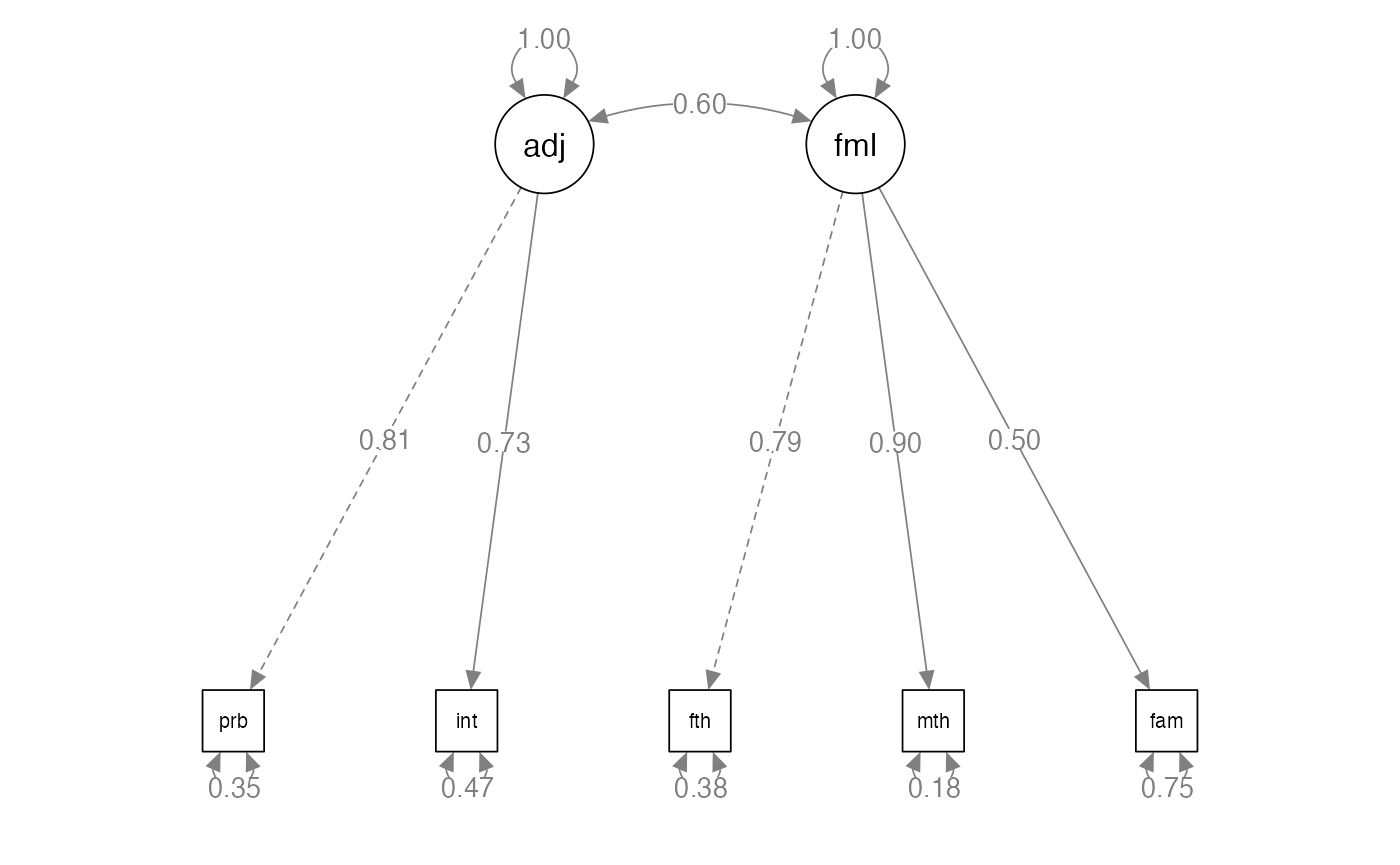
Example Model: Build Full SEM
predict.model <- '
adjust =~ problems + intimacy
family =~ father + mother + famo
adjust~family'
Example Model: Analyze Full SEM
predict.fit <- sem(model = predict.model,
                   sample.cov = family.cor,
                   sample.nobs = 203)
Example Model: Summarize Full SEM
summary(predict.fit,
        rsquare = TRUE,
        standardized = TRUE,
        fit.measures = TRUE)
#> lavaan 0.6-19 ended normally after 20 iterations
#>
#>   Estimator                                         ML
#>   Optimization method                           NLMINB
#>   Number of model parameters                        11
#>
#>   Number of observations                           203
#>
#> Model Test User Model:
#>
#>   Test statistic                               197.939
#>   Degrees of freedom                                 4
#>   P-value (Chi-square)                           0.000
#>
#> Model Test Baseline Model:
#>
#>   Test statistic                               533.051
#>   Degrees of freedom                                10
#>   P-value                                        0.000
#>
#> User Model versus Baseline Model:
#>
#>   Comparative Fit Index (CFI)                    0.629
#>   Tucker-Lewis Index (TLI)                       0.073
#>
#> Loglikelihood and Information Criteria:
#>
#>   Loglikelihood user model (H0)              -1270.160
#>   Loglikelihood unrestricted model (H1)      -1171.191
#>
#>   Akaike (AIC)                                2562.321
#>   Bayesian (BIC)                              2598.766
#>   Sample-size adjusted Bayesian (SABIC)       2563.915
#>
#> Root Mean Square Error of Approximation:
#>
#>   RMSEA                                          0.489
#>   90 Percent confidence interval - lower         0.432
#>   90 Percent confidence interval - upper         0.548
#>   P-value H_0: RMSEA <= 0.050                    0.000
#>   P-value H_0: RMSEA >= 0.080                    1.000
#>
#> Standardized Root Mean Square Residual:
#>
#>   SRMR                                           0.186
#>
#> Parameter Estimates:
#>
#>   Standard errors                             Standard
#>   Information                                 Expected
#>   Information saturated (h1) model          Structured
#>
#> Latent Variables:
#>                    Estimate  Std.Err  z-value  P(>|z|)   Std.lv  Std.all
#>   adjust =~
#>     problems          1.000                               0.807    0.809
#>     intimacy          0.901    0.134    6.741    0.000    0.727    0.729
#>   family =~
#>     father            1.000                               0.789    0.790
#>     mother            1.143    0.112   10.165    0.000    0.901    0.903
#>     famo              0.630    0.092    6.847    0.000    0.497    0.498
#>
#> Regressions:
#>                    Estimate  Std.Err  z-value  P(>|z|)   Std.lv  Std.all
#>   adjust ~
#>     family            0.618    0.092    6.705    0.000    0.604    0.604
#>
#> Variances:
#>                    Estimate  Std.Err  z-value  P(>|z|)   Std.lv  Std.all
#>    .problems          0.344    0.092    3.720    0.000    0.344    0.345
#>    .intimacy          0.466    0.084    5.571    0.000    0.466    0.468
#>    .father            0.373    0.062    6.035    0.000    0.373    0.375
#>    .mother            0.183    0.066    2.758    0.006    0.183    0.184
#>    .famo              0.748    0.079    9.530    0.000    0.748    0.752
#>    .adjust            0.414    0.095    4.364    0.000    0.636    0.636
#>     family            0.622    0.104    5.974    0.000    1.000    1.000
#>
#> R-Square:
#>                    Estimate
#>     problems          0.655
#>     intimacy          0.532
#>     father            0.625
#>     mother            0.816
#>     famo              0.248
#>     adjust            0.364
Example Model: Diagram Full SEM
semPaths(predict.fit,
         whatLabels="std",
         layout="tree",
         edge.label.cex = 1)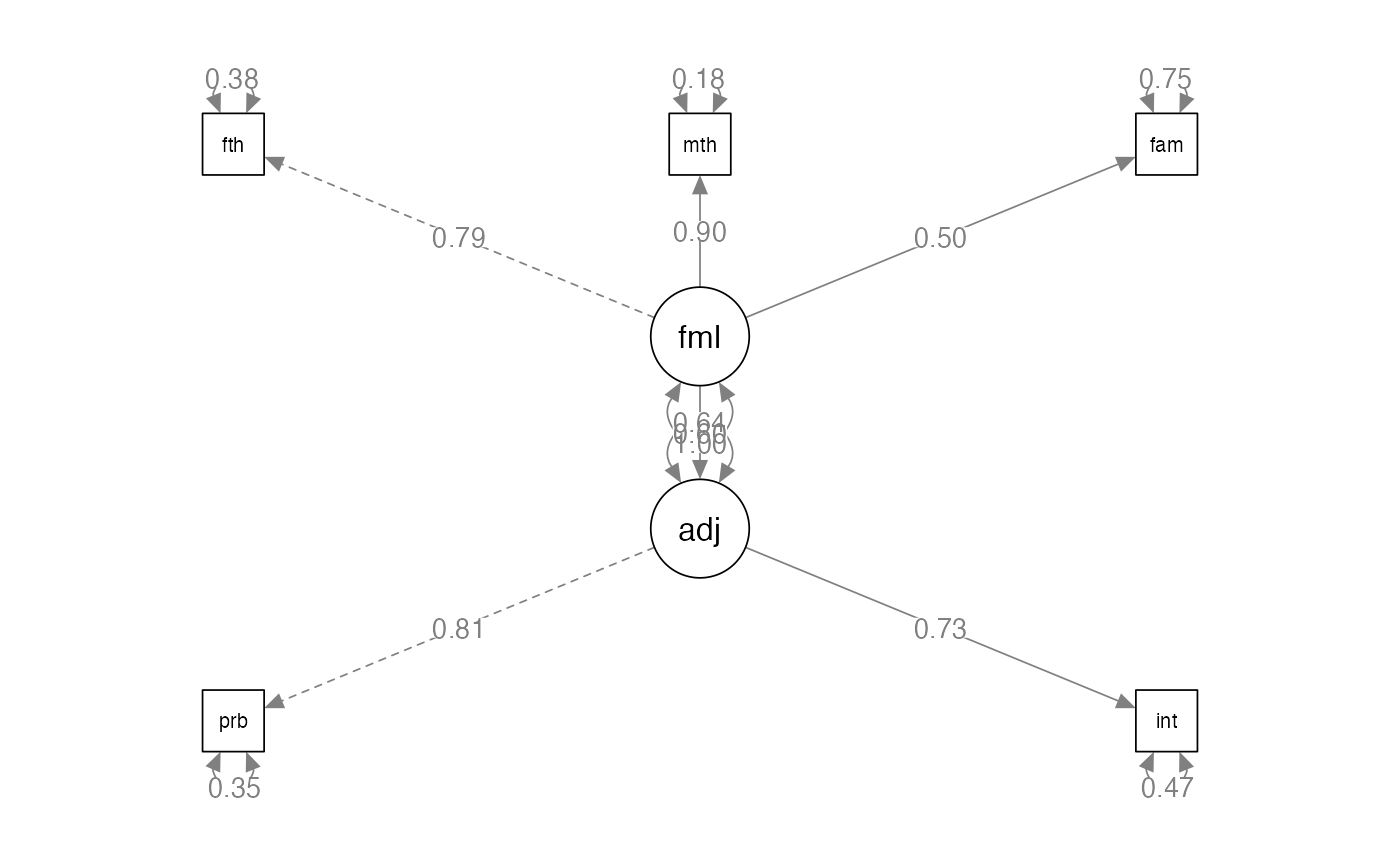
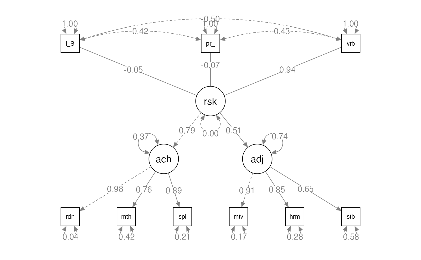
Example 2: Setup
family.cor <- lav_matrix_lower2full(c(1.00,
                                     .42,   1.00,
                                    -.43,   -.50,   1.00,
                                    -.39,   -.43,   .78,    1.00,
                                    -.24,   -.37,   .69,    .73,    1.00,
                                    -.31,   -.33,   .63,    .87,    .72,    1.00,
                                    -.25,   -.25,   .49,    .53,    .60,    .59,    1.00,
                                     -.25,  -.26,   .42,    .42,    .44,    .45,    .77,    1.00,
                                     -.16,  -.18,   .23,    .36,    .38,    .38,    .59,    .58, 1.00))

family.sd <- c(13.00,   13.50,  13.10,  12.50,  13.50,  14.20,  9.50,   11.10,  8.70)

rownames(family.cor) <-
  colnames(family.cor) <-
  names(family.sd) <- c("parent_psych","low_SES","verbal",
                        "reading","math","spelling","motivation","harmony","stable")

family.cov <- cor2cov(family.cor, family.sd)
Example 2: Build the Model
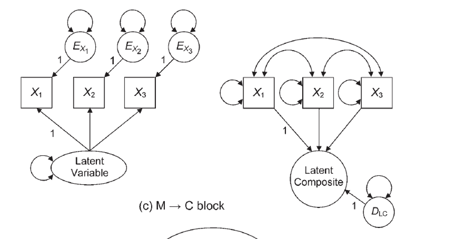
- How to define a composite variable?
- We have been using
=~to define a latent variable that predicts manifest variables. - Use
<~to create a composite variable that is predicted by the manifest variables.
Example 2: Build the Model
composite.model <- '
risk <~ low_SES + parent_psych + verbal
achieve =~ reading + math + spelling
adjustment =~ motivation + harmony + stable
risk =~ achieve + adjustment
'
Example 2: Analyze the Model
composite.fit <- sem(model = composite.model,
                      sample.cov = family.cov,
                      sample.nobs = 158)
Example 2: Summarize the Model
summary(composite.fit,
        rsquare = TRUE,
        standardized = TRUE,
        fit.measures = TRUE)
#> lavaan 0.6-19 ended normally after 78 iterations
#>
#>   Estimator                                         ML
#>   Optimization method                           NLMINB
#>   Number of model parameters                        16
#>
#>   Number of observations                           158
#>
#> Model Test User Model:
#>
#>   Test statistic                                94.965
#>   Degrees of freedom                                23
#>   P-value (Chi-square)                           0.000
#>
#> Model Test Baseline Model:
#>
#>   Test statistic                               852.585
#>   Degrees of freedom                                33
#>   P-value                                        0.000
#>
#> User Model versus Baseline Model:
#>
#>   Comparative Fit Index (CFI)                    0.912
#>   Tucker-Lewis Index (TLI)                       0.874
#>
#> Loglikelihood and Information Criteria:
#>
#>   Loglikelihood user model (H0)              -3270.643
#>   Loglikelihood unrestricted model (H1)      -3223.160
#>
#>   Akaike (AIC)                                6573.286
#>   Bayesian (BIC)                              6622.287
#>   Sample-size adjusted Bayesian (SABIC)       6571.640
#>
#> Root Mean Square Error of Approximation:
#>
#>   RMSEA                                          0.141
#>   90 Percent confidence interval - lower         0.112
#>   90 Percent confidence interval - upper         0.171
#>   P-value H_0: RMSEA <= 0.050                    0.000
#>   P-value H_0: RMSEA >= 0.080                    1.000
#>
#> Standardized Root Mean Square Residual:
#>
#>   SRMR                                           0.089
#>
#> Parameter Estimates:
#>
#>   Standard errors                             Standard
#>   Information                                 Expected
#>   Information saturated (h1) model          Structured
#>
#> Latent Variables:
#>                    Estimate  Std.Err  z-value  P(>|z|)   Std.lv  Std.all
#>   achieve =~
#>     reading           1.000                              12.183    0.978
#>     math              0.843    0.062   13.545    0.000   10.265    0.763
#>     spelling          1.030    0.053   19.583    0.000   12.546    0.886
#>   adjustment =~
#>     motivation        1.000                               8.632    0.912
#>     harmony           1.089    0.092   11.861    0.000    9.402    0.850
#>     stable            0.654    0.074    8.828    0.000    5.642    0.651
#>   risk =~
#>     achieve           1.000                               0.794    0.794
#>     adjustment        0.457    0.074    6.206    0.000    0.511    0.511
#>
#> Composites:
#>                    Estimate  Std.Err  z-value  P(>|z|)   Std.lv  Std.all
#>   risk <~
#>     low_SES          -0.033    0.050   -0.647    0.518   -0.003   -0.045
#>     parent_psych     -0.055    0.050   -1.095    0.274   -0.006   -0.074
#>     verbal            0.698    0.055   12.576    0.000    0.072    0.942
#>
#> Variances:
#>                    Estimate  Std.Err  z-value  P(>|z|)   Std.lv  Std.all
#>    .reading           6.831    3.848    1.775    0.076    6.831    0.044
#>    .math             75.732    9.120    8.304    0.000   75.732    0.418
#>    .spelling         42.954    6.357    6.757    0.000   42.954    0.214
#>    .motivation       15.162    4.920    3.082    0.002   15.162    0.169
#>    .harmony          34.034    6.723    5.062    0.000   34.034    0.278
#>    .stable           43.376    5.381    8.060    0.000   43.376    0.577
#>     risk              0.000                               0.000    0.000
#>    .achieve          54.931    7.452    7.372    0.000    0.370    0.370
#>    .adjustment       55.023    8.469    6.497    0.000    0.738    0.738
#>
#> R-Square:
#>                    Estimate
#>     reading           0.956
#>     math              0.582
#>     spelling          0.786
#>     motivation        0.831
#>     harmony           0.722
#>     stable            0.423
#>     achieve           0.630
#>     adjustment        0.262
Example 2: Improve the Model?
modificationindices(composite.fit, sort = T)
#>             lhs op          rhs     mi     epc sepc.lv sepc.all sepc.nox
#> 29         risk =~     spelling 22.091  -0.607  -5.874   -0.415   -0.415
#> 39      reading ~~         math 22.090 -27.301 -27.301   -1.200   -1.200
#> 54         risk ~~      achieve 15.658  42.911      NA       NA       NA
#> 56      achieve ~~   adjustment 15.658  19.593   0.356    0.356    0.356
#> 18         risk ~~         risk 15.658  42.911   0.000    0.000    0.000
#> 55         risk ~~   adjustment 15.658  19.593      NA       NA       NA
#> 37   adjustment =~         math 12.595   0.345   2.979    0.221    0.221
#> 33      achieve =~   motivation  8.857   0.140   1.710    0.181    0.181
#> 48     spelling ~~   motivation  8.351   8.974   8.974    0.352    0.352
#> 40      reading ~~     spelling  8.135  25.450  25.450    1.486    1.486
#> 28         risk =~         math  8.135   0.379   3.665    0.272    0.272
#> 45         math ~~   motivation  7.454  10.793  10.793    0.319    0.319
#> 38   adjustment =~     spelling  7.118   0.208   1.794    0.127    0.127
#> 44         math ~~     spelling  6.189  15.229  15.229    0.267    0.267
#> 27         risk =~      reading  6.189   0.320   3.090    0.248    0.248
#> 51   motivation ~~      harmony  4.044 -27.644 -27.644   -1.217   -1.217
#> 32         risk =~       stable  4.044  -0.138  -1.331   -0.153   -0.153
#> 41      reading ~~   motivation  3.494  -4.224  -4.224   -0.415   -0.415
#> 30         risk =~   motivation  2.929   0.122   1.183    0.125    0.125
#> 53      harmony ~~       stable  2.929  10.495  10.495    0.273    0.273
#> 43      reading ~~       stable  1.885   3.814   3.814    0.222    0.222
#> 36   adjustment =~      reading  1.618  -0.073  -0.634   -0.051   -0.051
#> 34      achieve =~      harmony  1.128  -0.059  -0.717   -0.065   -0.065
#> 46         math ~~      harmony  0.939  -4.694  -4.694   -0.092   -0.092
#> 31         risk =~      harmony  0.121  -0.028  -0.269   -0.024   -0.024
#> 52   motivation ~~       stable  0.121  -2.010  -2.010   -0.078   -0.078
#> 50     spelling ~~       stable  0.070   1.008   1.008    0.023    0.023
#> 49     spelling ~~      harmony  0.033  -0.687  -0.687   -0.018   -0.018
#> 42      reading ~~      harmony  0.021  -0.400  -0.400   -0.026   -0.026
#> 35      achieve =~       stable  0.017   0.007   0.082    0.009    0.009
#> 47         math ~~       stable  0.009   0.448   0.448    0.008    0.008
#> 58      low_SES  ~       verbal  0.000   0.000   0.000    0.000    0.000
#> 57      low_SES  ~ parent_psych  0.000   0.000   0.000    0.000    0.000
#> 60 parent_psych  ~       verbal  0.000   0.000   0.000    0.000    0.000
#> 59 parent_psych  ~      low_SES  0.000   0.000   0.000    0.000    0.000
#> 62       verbal  ~ parent_psych  0.000   0.000   0.000    0.000    0.000
#> 26       verbal ~~       verbal  0.000   0.000   0.000    0.000    0.000
#> 61       verbal  ~      low_SES  0.000   0.000   0.000    0.000    0.000
Example 2: Diagram the Model
semPaths(composite.fit,
         whatLabels="std",
         layout="tree",
         edge.label.cex = 1)