Exploratory Factor Analysis • learnSEM

Terminology

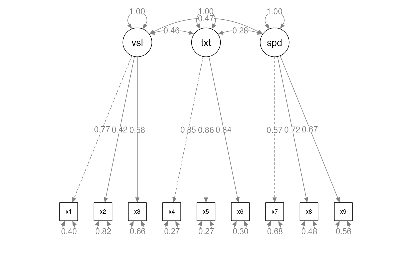
Measured variables – the real scores from the experiment
- Squares on a diagram
Latent variables – the construct the measured variables are supposed to represent
- Not measured directly
- Circles on a diagram

Terminology

What is EFA?

Factor analysis attempts to achieve parsimony (data reduction) by:
- Explaining the maximum amount of common variance in a correlation matrix
- Using the smallest number of explanatory constructs (factors)
Common variance is the overlapping variance between items
Unique variance is the variance only related to that item (error variance)

Directionality

Factors are thought to cause the measured variables
Therefore, we are saying that the measured variable is predicted by the factor

Why use EFA?

Understand structure of set of variables
Construct a scale to measure the latent variable
Reduce data set to smaller size that still measures original information

The Example Data

We are going to build a scale that measures the anxiety that statistics provokes in students
Dataset is from the Field textbook

Statistics makes me cry
My friends will think I’m stupid for not being able to cope with R
Standard deviations excite me
I dream that Pearson is attacking me with correlation coefficients
I don’t understand statistics
I have little experience of computers
All computers hate me
I have never been good at mathematics
My friends are better at statistics than me
Computers are useful only for playing games
I did badly at mathematics at school
People try to tell you that R makes statistics easier to understand but it doesn’t
I worry that I will cause irreparable damage because of my incompetence with computers
Computers have minds of their own and deliberately go wrong whenever I use them
Computers are out to get me
I weep openly at the mention of central tendency
I slip into a coma whenever I see an equation
R always crashes when I try to use it
Everybody looks at me when I use R
I can’t sleep for thoughts of eigenvectors
I wake up under my duvet thinking that I am trapped under a normal distribution
My friends are better at R than I am
If I’m good at statistics my friends will think I’m a nerd

The Example Data

library(rio)
library(psych)
master <- import("data/lecture_efa.csv")
head(master)
#>   Q01 Q02 Q03 Q04 Q05 Q06 Q07 Q08 Q09 Q10 Q11 Q12 Q13 Q14 Q15 Q16 Q17 Q18 Q19
#> 1   4   5   2   4   4   4   3   5   5   4   5   4   4   4   4   3   5   4   3
#> 2   5   5   2   3   4   4   4   4   1   4   4   3   5   3   2   3   4   4   3
#> 3   4   3   4   4   2   5   4   4   4   4   3   3   4   2   4   3   4   3   5
#> 4   3   5   5   2   3   3   2   4   4   2   4   4   4   3   3   3   4   2   4
#> 5   4   5   3   4   4   3   3   4   2   4   4   3   3   4   4   4   4   3   3
#> 6   4   5   3   4   2   2   2   4   2   3   4   2   3   3   1   4   3   1   5
#>   Q20 Q21 Q22 Q23
#> 1   4   4   4   1
#> 2   2   2   2   4
#> 3   2   3   4   4
#> 4   2   2   2   3
#> 5   2   4   2   2
#> 6   1   3   5   2

Steps to Analysis

Data screening (not shown, use last week’s notes!)
- Additionally, you need at least interval measurement for the analyses shown here
- Enough items to group into factors (recommended 3-4 per potential factor)
How many factors should you use?
Simple structure
Adequate solutions

How many factors do I use?

Theory
Kaiser criterion
Scree plots
Parallel analysis

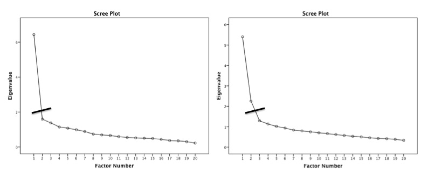
Kaiser criterion

Old rule: extract the number of eigenvalues over 1
New rule: extract the number of eigenvalues over .7
What the heck is an eigenvalue?
- A mathematical representation of the variance accounted for by that grouping of items

Scree plots

Parallel analysis

A statistical test to tell you how many eigenvalues are greater than chance
- Calculates the eigenvalues for your data
- Randomizes your data and recalculates the eigenvalues
- Then compares them to determine if they are equal

Finding factors/components

number_items <- fa.parallel(master, #data frame
                            fm="ml", #math
                            fa="fa") #only efa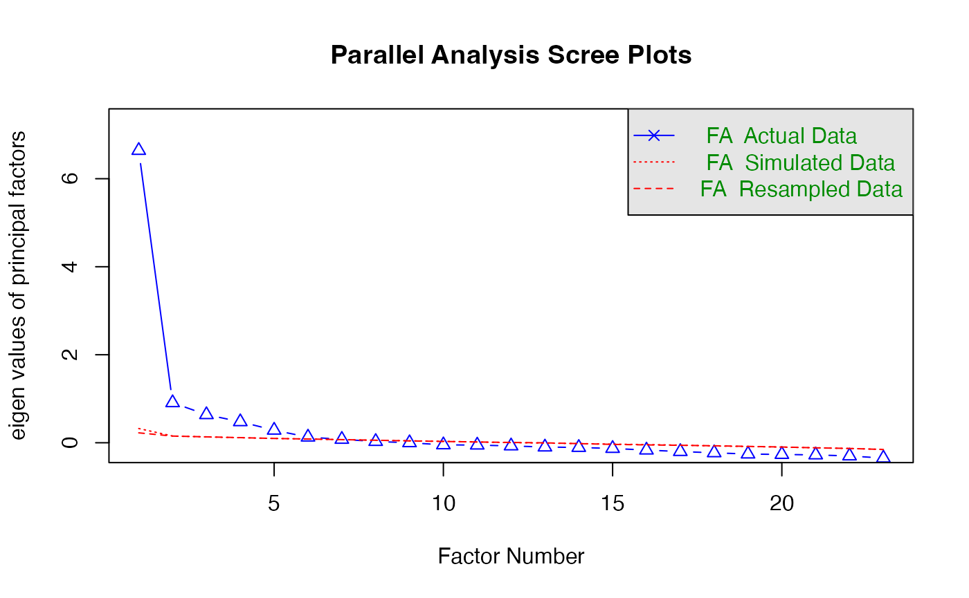

#> Parallel analysis suggests that the number of factors =  6  and the number of components =  NA

Eigenvalues

 
sum(number_items$fa.values > 1)
#> [1] 1
sum(number_items$fa.values > .7)
#> [1] 2

Simple structure

Simple structure covers two pieces:
- The math used to achieve the solution: maximum likelihood
- Rotation to increase communality between items and aid in interpretation

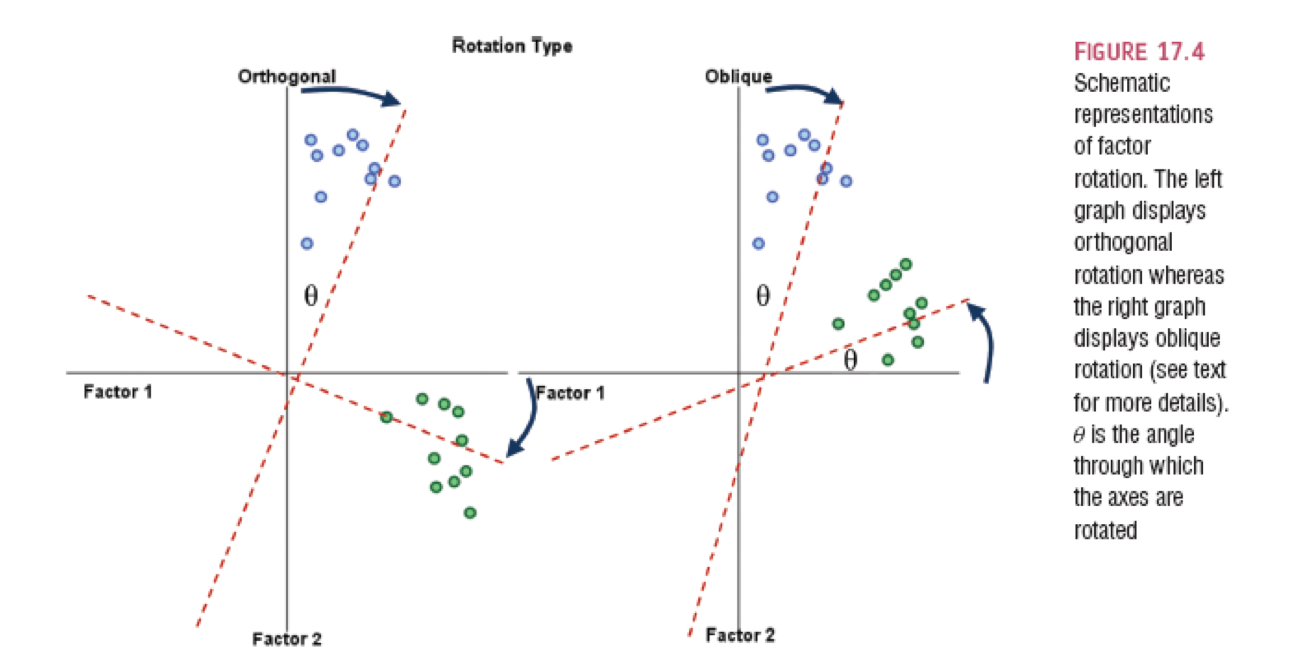
Rotation

Orthogonal assume uncorrelated factors: varimax, quartermax, equamax
Oblique allows factors to be correlated: oblimin, promax
Why would we even use orthogonal?

Simple structure/solution

Looking at the loadings: the relationship between the item and the factor/component
- Want these to be related at least .3
- Remember that r = .3 is a medium effect size that is ~10% variance
- Can eliminate items that load poorly
- Difference here in scale development versus exploratory clustering

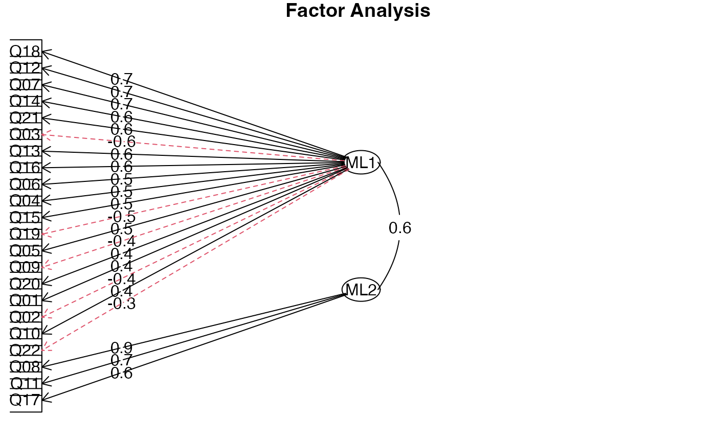
Run an EFA

EFA_fit <- fa(master, #data
              nfactors = 2, #number of factors
              rotate = "oblimin", #rotation
              fm = "ml") #math
#> Loading required namespace: GPArotation

Look at the results

EFA_fit
#> Factor Analysis using method =  ml
#> Call: fa(r = master, nfactors = 2, rotate = "oblimin", fm = "ml")
#> Standardized loadings (pattern matrix) based upon correlation matrix
#>       ML1   ML2    h2   u2 com
#> Q01  0.41  0.21 0.310 0.69 1.5
#> Q02 -0.40  0.17 0.111 0.89 1.3
#> Q03 -0.62  0.02 0.369 0.63 1.0
#> Q04  0.49  0.17 0.366 0.63 1.2
#> Q05  0.45  0.10 0.269 0.73 1.1
#> Q06  0.55  0.00 0.301 0.70 1.0
#> Q07  0.66  0.02 0.454 0.55 1.0
#> Q08 -0.08  0.86 0.670 0.33 1.0
#> Q09 -0.44  0.25 0.128 0.87 1.6
#> Q10  0.40  0.02 0.167 0.83 1.0
#> Q11  0.16  0.66 0.593 0.41 1.1
#> Q12  0.70 -0.05 0.446 0.55 1.0
#> Q13  0.60  0.09 0.429 0.57 1.0
#> Q14  0.64  0.00 0.415 0.58 1.0
#> Q15  0.47  0.13 0.313 0.69 1.1
#> Q16  0.58  0.11 0.418 0.58 1.1
#> Q17  0.17  0.64 0.570 0.43 1.1
#> Q18  0.71 -0.02 0.493 0.51 1.0
#> Q19 -0.47  0.09 0.177 0.82 1.1
#> Q20  0.42 -0.01 0.169 0.83 1.0
#> Q21  0.62  0.03 0.407 0.59 1.0
#> Q22 -0.34  0.09 0.090 0.91 1.2
#> Q23 -0.15  0.03 0.018 0.98 1.1
#> 
#>                        ML1  ML2
#> SS loadings           5.70 1.98
#> Proportion Var        0.25 0.09
#> Cumulative Var        0.25 0.33
#> Proportion Explained  0.74 0.26
#> Cumulative Proportion 0.74 1.00
#> 
#>  With factor correlations of 
#>      ML1  ML2
#> ML1 1.00 0.58
#> ML2 0.58 1.00
#> 
#> Mean item complexity =  1.1
#> Test of the hypothesis that 2 factors are sufficient.
#> 
#> df null model =  253  with the objective function =  7.55 with Chi Square =  19334.49
#> df of  the model are 208  and the objective function was  1.13 
#> 
#> The root mean square of the residuals (RMSR) is  0.05 
#> The df corrected root mean square of the residuals is  0.06 
#> 
#> The harmonic n.obs is  2571 with the empirical chi square  3481.13  with prob <  0 
#> The total n.obs was  2571  with Likelihood Chi Square =  2893.46  with prob <  0 
#> 
#> Tucker Lewis Index of factoring reliability =  0.829
#> RMSEA index =  0.071  and the 90 % confidence intervals are  0.069 0.073
#> BIC =  1260.24
#> Fit based upon off diagonal values = 0.97
#> Measures of factor score adequacy             
#>                                                    ML1  ML2
#> Correlation of (regression) scores with factors   0.95 0.91
#> Multiple R square of scores with factors          0.90 0.84
#> Minimum correlation of possible factor scores     0.81 0.67

Item 23

EFA_fit2 <- fa(master[ , -23], #data
              nfactors = 2, #number of factors
              rotate = "oblimin", #rotation
              fm = "ml") #math

EFA_fit2
#> Factor Analysis using method =  ml
#> Call: fa(r = master[, -23], nfactors = 2, rotate = "oblimin", fm = "ml")
#> Standardized loadings (pattern matrix) based upon correlation matrix
#>       ML1   ML2    h2   u2 com
#> Q01  0.41  0.20 0.311 0.69 1.5
#> Q02 -0.40  0.16 0.108 0.89 1.3
#> Q03 -0.61  0.01 0.367 0.63 1.0
#> Q04  0.49  0.17 0.367 0.63 1.2
#> Q05  0.45  0.10 0.270 0.73 1.1
#> Q06  0.55  0.00 0.302 0.70 1.0
#> Q07  0.67  0.01 0.455 0.55 1.0
#> Q08 -0.08  0.86 0.672 0.33 1.0
#> Q09 -0.43  0.24 0.123 0.88 1.6
#> Q10  0.40  0.02 0.167 0.83 1.0
#> Q11  0.16  0.66 0.594 0.41 1.1
#> Q12  0.70 -0.05 0.448 0.55 1.0
#> Q13  0.60  0.09 0.430 0.57 1.0
#> Q14  0.65  0.00 0.417 0.58 1.0
#> Q15  0.47  0.13 0.313 0.69 1.1
#> Q16  0.58  0.11 0.418 0.58 1.1
#> Q17  0.17  0.64 0.570 0.43 1.1
#> Q18  0.72 -0.02 0.494 0.51 1.0
#> Q19 -0.46  0.09 0.175 0.82 1.1
#> Q20  0.42 -0.01 0.169 0.83 1.0
#> Q21  0.62  0.03 0.407 0.59 1.0
#> Q22 -0.34  0.09 0.086 0.91 1.1
#> 
#>                        ML1  ML2
#> SS loadings           5.68 1.98
#> Proportion Var        0.26 0.09
#> Cumulative Var        0.26 0.35
#> Proportion Explained  0.74 0.26
#> Cumulative Proportion 0.74 1.00
#> 
#>  With factor correlations of 
#>      ML1  ML2
#> ML1 1.00 0.58
#> ML2 0.58 1.00
#> 
#> Mean item complexity =  1.1
#> Test of the hypothesis that 2 factors are sufficient.
#> 
#> df null model =  231  with the objective function =  7.46 with Chi Square =  19107.61
#> df of  the model are 188  and the objective function was  1.06 
#> 
#> The root mean square of the residuals (RMSR) is  0.05 
#> The df corrected root mean square of the residuals is  0.06 
#> 
#> The harmonic n.obs is  2571 with the empirical chi square  3094.97  with prob <  0 
#> The total n.obs was  2571  with Likelihood Chi Square =  2705.25  with prob <  0 
#> 
#> Tucker Lewis Index of factoring reliability =  0.836
#> RMSEA index =  0.072  and the 90 % confidence intervals are  0.07 0.075
#> BIC =  1229.07
#> Fit based upon off diagonal values = 0.97
#> Measures of factor score adequacy             
#>                                                    ML1  ML2
#> Correlation of (regression) scores with factors   0.95 0.91
#> Multiple R square of scores with factors          0.90 0.84
#> Minimum correlation of possible factor scores     0.81 0.67

Plots of the results

The built in plot functions from psych are fantastic!

 fa.plot(EFA_fit2, 
     labels = colnames(master[ , -23]))

Plots of the results

fa.diagram(EFA_fit2)

Adequate solution

Fit indices: a measure of how well the model matches the data
- Goodness of fit statistics: measure the overlap between the reproduced correlation matrix and the original, want high numbers close to 1
- Badness of fit statistics (residual): measure the mismatch, want low numbers close to zero
Theory/interpretability
Reliability

Fit statistics

EFA_fit2$rms #Root mean square of the residuals
#> [1] 0.05104534
EFA_fit2$RMSEA #root mean squared error of approximation
#>      RMSEA      lower      upper confidence 
#> 0.07216508 0.06978342 0.07460328 0.90000000
EFA_fit2$TLI #tucker lewis index
#> [1] 0.8360597
1 - ((EFA_fit2$STATISTIC-EFA_fit2$dof)/
       (EFA_fit2$null.chisq-EFA_fit2$null.dof)) #CFI 
#> [1] 0.866647

Reliability

factor1 = c(1:7, 9:10, 12:16, 18:22)
factor2 = c(8, 11, 17)
##we use the psych::alpha to make sure that R knows we want the alpha function from the psych package.
##ggplot2 has an alpha function and if we have them both open at the same time
##you will sometimes get a color error without this :: information. 
psych::alpha(master[, factor1], check.keys = T)
#> Warning in psych::alpha(master[, factor1], check.keys = T): Some items were negatively correlated with the first principal component and were automatically reversed.
#>  This is indicated by a negative sign for the variable name.
#> 
#> Reliability analysis   
#> Call: psych::alpha(x = master[, factor1], check.keys = T)
#> 
#>   raw_alpha std.alpha G6(smc) average_r S/N    ase mean   sd median_r
#>       0.88      0.88    0.89      0.28 7.4 0.0034    3 0.56     0.27
#> 
#>     95% confidence boundaries 
#>          lower alpha upper
#> Feldt     0.87  0.88  0.89
#> Duhachek  0.87  0.88  0.89
#> 
#>  Reliability if an item is dropped:
#>      raw_alpha std.alpha G6(smc) average_r S/N alpha se var.r med.r
#> Q01       0.87      0.88    0.88      0.28 7.0   0.0036 0.013  0.27
#> Q02-      0.88      0.88    0.89      0.29 7.5   0.0035 0.013  0.30
#> Q03-      0.87      0.87    0.88      0.28 6.8   0.0037 0.014  0.26
#> Q04       0.87      0.87    0.88      0.28 6.9   0.0037 0.013  0.27
#> Q05       0.87      0.88    0.89      0.28 7.1   0.0036 0.014  0.27
#> Q06       0.87      0.88    0.88      0.28 7.0   0.0036 0.013  0.27
#> Q07       0.87      0.87    0.88      0.27 6.8   0.0038 0.013  0.26
#> Q09-      0.88      0.88    0.89      0.29 7.5   0.0033 0.013  0.30
#> Q10       0.88      0.88    0.89      0.29 7.3   0.0035 0.014  0.30
#> Q12       0.87      0.87    0.88      0.27 6.8   0.0037 0.013  0.26
#> Q13       0.87      0.87    0.88      0.27 6.8   0.0037 0.013  0.27
#> Q14       0.87      0.87    0.88      0.27 6.8   0.0037 0.013  0.27
#> Q15       0.87      0.87    0.88      0.28 7.0   0.0036 0.014  0.27
#> Q16       0.87      0.87    0.88      0.27 6.8   0.0037 0.013  0.26
#> Q18       0.87      0.87    0.88      0.27 6.7   0.0038 0.012  0.27
#> Q19-      0.88      0.88    0.89      0.29 7.2   0.0035 0.014  0.30
#> Q20       0.88      0.88    0.89      0.29 7.3   0.0035 0.014  0.30
#> Q21       0.87      0.87    0.88      0.27 6.8   0.0037 0.013  0.26
#> Q22-      0.88      0.88    0.89      0.29 7.5   0.0034 0.013  0.30
#> 
#>  Item statistics 
#>         n raw.r std.r r.cor r.drop mean   sd
#> Q01  2571  0.55  0.57  0.54   0.49  3.6 0.83
#> Q02- 2571  0.38  0.38  0.33   0.31  1.6 0.85
#> Q03- 2571  0.65  0.65  0.62   0.59  2.6 1.08
#> Q04  2571  0.60  0.61  0.59   0.54  3.2 0.95
#> Q05  2571  0.55  0.56  0.52   0.48  3.3 0.96
#> Q06  2571  0.57  0.56  0.54   0.49  3.8 1.12
#> Q07  2571  0.68  0.68  0.66   0.62  3.1 1.10
#> Q09- 2571  0.40  0.38  0.32   0.30  2.8 1.26
#> Q10  2571  0.45  0.46  0.41   0.38  3.7 0.88
#> Q12  2571  0.67  0.67  0.66   0.61  2.8 0.92
#> Q13  2571  0.65  0.65  0.64   0.59  3.6 0.95
#> Q14  2571  0.65  0.65  0.63   0.59  3.1 1.00
#> Q15  2571  0.59  0.59  0.55   0.52  3.2 1.01
#> Q16  2571  0.66  0.67  0.66   0.61  3.1 0.92
#> Q18  2571  0.69  0.69  0.68   0.64  3.4 1.05
#> Q19- 2571  0.49  0.48  0.43   0.41  2.3 1.10
#> Q20  2571  0.47  0.47  0.42   0.39  2.4 1.04
#> Q21  2571  0.65  0.65  0.64   0.59  2.8 0.98
#> Q22- 2571  0.38  0.37  0.31   0.29  2.9 1.04
#> 
#> Non missing response frequency for each item
#>        1    2    3    4    5 miss
#> Q01 0.02 0.07 0.29 0.52 0.11    0
#> Q02 0.01 0.04 0.08 0.31 0.56    0
#> Q03 0.03 0.17 0.34 0.26 0.19    0
#> Q04 0.05 0.17 0.36 0.37 0.05    0
#> Q05 0.04 0.18 0.29 0.43 0.06    0
#> Q06 0.06 0.10 0.13 0.44 0.27    0
#> Q07 0.09 0.24 0.26 0.34 0.07    0
#> Q09 0.08 0.28 0.23 0.20 0.20    0
#> Q10 0.02 0.10 0.18 0.57 0.14    0
#> Q12 0.09 0.23 0.46 0.20 0.02    0
#> Q13 0.03 0.12 0.25 0.48 0.12    0
#> Q14 0.07 0.18 0.38 0.31 0.06    0
#> Q15 0.06 0.18 0.30 0.39 0.07    0
#> Q16 0.06 0.16 0.42 0.33 0.04    0
#> Q18 0.06 0.12 0.31 0.37 0.14    0
#> Q19 0.02 0.15 0.22 0.33 0.29    0
#> Q20 0.22 0.37 0.25 0.15 0.02    0
#> Q21 0.09 0.29 0.34 0.26 0.02    0
#> Q22 0.05 0.26 0.34 0.26 0.10    0
psych::alpha(master[, factor2], check.keys = T)
#> 
#> Reliability analysis   
#> Call: psych::alpha(x = master[, factor2], check.keys = T)
#> 
#>   raw_alpha std.alpha G6(smc) average_r S/N    ase mean   sd median_r
#>       0.82      0.82    0.75       0.6 4.5 0.0062  3.7 0.75     0.59
#> 
#>     95% confidence boundaries 
#>          lower alpha upper
#> Feldt     0.81  0.82  0.83
#> Duhachek  0.81  0.82  0.83
#> 
#>  Reliability if an item is dropped:
#>     raw_alpha std.alpha G6(smc) average_r S/N alpha se var.r med.r
#> Q08      0.74      0.74    0.59      0.59 2.8    0.010    NA  0.59
#> Q11      0.74      0.74    0.59      0.59 2.9    0.010    NA  0.59
#> Q17      0.77      0.77    0.63      0.63 3.4    0.009    NA  0.63
#> 
#>  Item statistics 
#>        n raw.r std.r r.cor r.drop mean   sd
#> Q08 2571  0.86  0.86  0.76   0.68  3.8 0.87
#> Q11 2571  0.86  0.86  0.75   0.68  3.7 0.88
#> Q17 2571  0.85  0.85  0.72   0.65  3.5 0.88
#> 
#> Non missing response frequency for each item
#>        1    2    3    4    5 miss
#> Q08 0.03 0.06 0.19 0.58 0.15    0
#> Q11 0.02 0.06 0.22 0.53 0.16    0
#> Q17 0.03 0.10 0.27 0.52 0.08    0

Interpretation

Factor 1:

Statistics makes me cry
My friends will think I’m stupid for not being able to cope with R
Standard deviations excite me
I dream that Pearson is attacking me with correlation coefficients
I don’t understand statistics
I have little experience of computers
All computers hate me
My friends are better at statistics than me
Computers are useful only for playing games
People try to tell you that R makes statistics easier to understand but it doesn’t
I worry that I will cause irreparable damage because of my incompetence with computers
Computers have minds of their own and deliberately go wrong whenever I use them
Computers are out to get me
I weep openly at the mention of central tendency
R always crashes when I try to use it
Everybody looks at me when I use R
I can’t sleep for thoughts of eigenvectors
I wake up under my duvet thinking that I am trapped under a normal distribution
My friends are better at R than I am

Factor 2:

I have never been good at mathematics
I did badly at mathematics at school
I slip into a coma whenever I see an equation

Bad:

If I’m good at statistics my friends will think I’m a nerd

Wrapping Up

You’ve learned about exploratory factor analysis, which we will revisit when we cover confirmatory factor analysis
You learned how to examine for the number of possible latent variables
You learned how to determine simple structure
You learned how to determine if that simple structure was an adequate model