Introduction to R • learnSEM

Overall Note

You can learn R.
You will get frustrated.
You will get errors that don’t help or make sense.
- Google is your friend.
- Try Googling the specific error message first.
- Then try googling your specific function and the error.
- Try a bunch of different search terms.

Helpful Websites

Quick-R: www.statmethods.net
R documentation: www.rdocumentation.org
Swirl: www.swirlstats.com
Stack Overflow: www.stackoverflow.com
Learn Statistics with R: https://learningstatisticswithr.com/

Download Requirements

Get R: http://cran.r-project.org/
Mac: XQuartz https://www.xquartz.org/ (if you find you do not have it)
RStudio: http://www.rstudio.org/

Outline

Commands
Object Types
Subsetting
Missing Data
Working Directories
Packages
Functions

Commands

Commands are the code that you tell R to do for you.
They can be very simple or complex.
Computers do what you tell them to do. Mistakes happen!
- Maybe it’s a typo, maybe it’s a misunderstanding of what the code does

Commands

You can type a command directly into the console
You can type in a document (Script or Markdown) and tell it to then run in the console

X <- 4

Commands

> indicates the console is ready for more code
+ indicates that you haven’t finished a code block
Capitalization and symbols matter
= and <- are equivalent
Hit the up arrow – you can scroll through the last commands that were run
Hit the tab key – you’ll get a list of variable names and options to select from
Use the ? followed by a command to learn more about it

Commands

Let’s take a look and run some simple commands
- Where is the console
- How do I move them around?
- How do I run code?
- What is a Script?
- What is Markdown?
- How do I run code in those?

RStudio

What are all the windows in RStudio?
Working Area:
- Current files that are open like scripts, markdown, etc.
Console, Terminal, Jobs
- Where the magic happens
- Where everything runs
Environment, History, …others
- Tells you what is saved in your working environment
- What variables and types of variables you have made
- Allows you to click to view them
Files, Plots, Packages, Help, Viewer
- Shows you a file viewer, pictures/plots, packages, and help!

Object Types

Here are some of the basics:
- Vectors
- Lists
- Matrices
- Data Frames
Within those objects, values can be:
- Character
- Factor (a special type of character)
- Numeric/Integer/Complex
- Logical (True, False)
- NaN (versus NA)
Last, objects can have attributes (names)

Objects Example

library(palmerpenguins)
data(penguins)
attributes(penguins)
#> $class
#> [1] "tbl_df"     "tbl"        "data.frame"
#> 
#> $row.names
#>   [1]   1   2   3   4   5   6   7   8   9  10  11  12  13  14  15  16  17  18
#>  [19]  19  20  21  22  23  24  25  26  27  28  29  30  31  32  33  34  35  36
#>  [37]  37  38  39  40  41  42  43  44  45  46  47  48  49  50  51  52  53  54
#>  [55]  55  56  57  58  59  60  61  62  63  64  65  66  67  68  69  70  71  72
#>  [73]  73  74  75  76  77  78  79  80  81  82  83  84  85  86  87  88  89  90
#>  [91]  91  92  93  94  95  96  97  98  99 100 101 102 103 104 105 106 107 108
#> [109] 109 110 111 112 113 114 115 116 117 118 119 120 121 122 123 124 125 126
#> [127] 127 128 129 130 131 132 133 134 135 136 137 138 139 140 141 142 143 144
#> [145] 145 146 147 148 149 150 151 152 153 154 155 156 157 158 159 160 161 162
#> [163] 163 164 165 166 167 168 169 170 171 172 173 174 175 176 177 178 179 180
#> [181] 181 182 183 184 185 186 187 188 189 190 191 192 193 194 195 196 197 198
#> [199] 199 200 201 202 203 204 205 206 207 208 209 210 211 212 213 214 215 216
#> [217] 217 218 219 220 221 222 223 224 225 226 227 228 229 230 231 232 233 234
#> [235] 235 236 237 238 239 240 241 242 243 244 245 246 247 248 249 250 251 252
#> [253] 253 254 255 256 257 258 259 260 261 262 263 264 265 266 267 268 269 270
#> [271] 271 272 273 274 275 276 277 278 279 280 281 282 283 284 285 286 287 288
#> [289] 289 290 291 292 293 294 295 296 297 298 299 300 301 302 303 304 305 306
#> [307] 307 308 309 310 311 312 313 314 315 316 317 318 319 320 321 322 323 324
#> [325] 325 326 327 328 329 330 331 332 333 334 335 336 337 338 339 340 341 342
#> [343] 343 344
#> 
#> $names
#> [1] "species"           "island"            "bill_length_mm"   
#> [4] "bill_depth_mm"     "flipper_length_mm" "body_mass_g"      
#> [7] "sex"               "year"

Objects Example

str(penguins)
#> tibble [344 × 8] (S3: tbl_df/tbl/data.frame)
#>  $ species          : Factor w/ 3 levels "Adelie","Chinstrap",..: 1 1 1 1 1 1 1 1 1 1 ...
#>  $ island           : Factor w/ 3 levels "Biscoe","Dream",..: 3 3 3 3 3 3 3 3 3 3 ...
#>  $ bill_length_mm   : num [1:344] 39.1 39.5 40.3 NA 36.7 39.3 38.9 39.2 34.1 42 ...
#>  $ bill_depth_mm    : num [1:344] 18.7 17.4 18 NA 19.3 20.6 17.8 19.6 18.1 20.2 ...
#>  $ flipper_length_mm: int [1:344] 181 186 195 NA 193 190 181 195 193 190 ...
#>  $ body_mass_g      : int [1:344] 3750 3800 3250 NA 3450 3650 3625 4675 3475 4250 ...
#>  $ sex              : Factor w/ 2 levels "female","male": 2 1 1 NA 1 2 1 2 NA NA ...
#>  $ year             : int [1:344] 2007 2007 2007 2007 2007 2007 2007 2007 2007 2007 ...

names(penguins) #ls(penguins) provides this as well 
#> [1] "species"           "island"            "bill_length_mm"   
#> [4] "bill_depth_mm"     "flipper_length_mm" "body_mass_g"      
#> [7] "sex"               "year"

Vectors

You can think about a vector as one row or column of data
All the objects must be the same class
If you try to mix and match, it will coerce them into the same type or make them NA if not.

X
#> [1] 4

[1] indicates the number of the first item for each printed row

penguins$species
#>   [1] Adelie    Adelie    Adelie    Adelie    Adelie    Adelie    Adelie   
#>   [8] Adelie    Adelie    Adelie    Adelie    Adelie    Adelie    Adelie   
#>  [15] Adelie    Adelie    Adelie    Adelie    Adelie    Adelie    Adelie   
#>  [22] Adelie    Adelie    Adelie    Adelie    Adelie    Adelie    Adelie   
#>  [29] Adelie    Adelie    Adelie    Adelie    Adelie    Adelie    Adelie   
#>  [36] Adelie    Adelie    Adelie    Adelie    Adelie    Adelie    Adelie   
#>  [43] Adelie    Adelie    Adelie    Adelie    Adelie    Adelie    Adelie   
#>  [50] Adelie    Adelie    Adelie    Adelie    Adelie    Adelie    Adelie   
#>  [57] Adelie    Adelie    Adelie    Adelie    Adelie    Adelie    Adelie   
#>  [64] Adelie    Adelie    Adelie    Adelie    Adelie    Adelie    Adelie   
#>  [71] Adelie    Adelie    Adelie    Adelie    Adelie    Adelie    Adelie   
#>  [78] Adelie    Adelie    Adelie    Adelie    Adelie    Adelie    Adelie   
#>  [85] Adelie    Adelie    Adelie    Adelie    Adelie    Adelie    Adelie   
#>  [92] Adelie    Adelie    Adelie    Adelie    Adelie    Adelie    Adelie   
#>  [99] Adelie    Adelie    Adelie    Adelie    Adelie    Adelie    Adelie   
#> [106] Adelie    Adelie    Adelie    Adelie    Adelie    Adelie    Adelie   
#> [113] Adelie    Adelie    Adelie    Adelie    Adelie    Adelie    Adelie   
#> [120] Adelie    Adelie    Adelie    Adelie    Adelie    Adelie    Adelie   
#> [127] Adelie    Adelie    Adelie    Adelie    Adelie    Adelie    Adelie   
#> [134] Adelie    Adelie    Adelie    Adelie    Adelie    Adelie    Adelie   
#> [141] Adelie    Adelie    Adelie    Adelie    Adelie    Adelie    Adelie   
#> [148] Adelie    Adelie    Adelie    Adelie    Adelie    Gentoo    Gentoo   
#> [155] Gentoo    Gentoo    Gentoo    Gentoo    Gentoo    Gentoo    Gentoo   
#> [162] Gentoo    Gentoo    Gentoo    Gentoo    Gentoo    Gentoo    Gentoo   
#> [169] Gentoo    Gentoo    Gentoo    Gentoo    Gentoo    Gentoo    Gentoo   
#> [176] Gentoo    Gentoo    Gentoo    Gentoo    Gentoo    Gentoo    Gentoo   
#> [183] Gentoo    Gentoo    Gentoo    Gentoo    Gentoo    Gentoo    Gentoo   
#> [190] Gentoo    Gentoo    Gentoo    Gentoo    Gentoo    Gentoo    Gentoo   
#> [197] Gentoo    Gentoo    Gentoo    Gentoo    Gentoo    Gentoo    Gentoo   
#> [204] Gentoo    Gentoo    Gentoo    Gentoo    Gentoo    Gentoo    Gentoo   
#> [211] Gentoo    Gentoo    Gentoo    Gentoo    Gentoo    Gentoo    Gentoo   
#> [218] Gentoo    Gentoo    Gentoo    Gentoo    Gentoo    Gentoo    Gentoo   
#> [225] Gentoo    Gentoo    Gentoo    Gentoo    Gentoo    Gentoo    Gentoo   
#> [232] Gentoo    Gentoo    Gentoo    Gentoo    Gentoo    Gentoo    Gentoo   
#> [239] Gentoo    Gentoo    Gentoo    Gentoo    Gentoo    Gentoo    Gentoo   
#> [246] Gentoo    Gentoo    Gentoo    Gentoo    Gentoo    Gentoo    Gentoo   
#> [253] Gentoo    Gentoo    Gentoo    Gentoo    Gentoo    Gentoo    Gentoo   
#> [260] Gentoo    Gentoo    Gentoo    Gentoo    Gentoo    Gentoo    Gentoo   
#> [267] Gentoo    Gentoo    Gentoo    Gentoo    Gentoo    Gentoo    Gentoo   
#> [274] Gentoo    Gentoo    Gentoo    Chinstrap Chinstrap Chinstrap Chinstrap
#> [281] Chinstrap Chinstrap Chinstrap Chinstrap Chinstrap Chinstrap Chinstrap
#> [288] Chinstrap Chinstrap Chinstrap Chinstrap Chinstrap Chinstrap Chinstrap
#> [295] Chinstrap Chinstrap Chinstrap Chinstrap Chinstrap Chinstrap Chinstrap
#> [302] Chinstrap Chinstrap Chinstrap Chinstrap Chinstrap Chinstrap Chinstrap
#> [309] Chinstrap Chinstrap Chinstrap Chinstrap Chinstrap Chinstrap Chinstrap
#> [316] Chinstrap Chinstrap Chinstrap Chinstrap Chinstrap Chinstrap Chinstrap
#> [323] Chinstrap Chinstrap Chinstrap Chinstrap Chinstrap Chinstrap Chinstrap
#> [330] Chinstrap Chinstrap Chinstrap Chinstrap Chinstrap Chinstrap Chinstrap
#> [337] Chinstrap Chinstrap Chinstrap Chinstrap Chinstrap Chinstrap Chinstrap
#> [344] Chinstrap
#> Levels: Adelie Chinstrap Gentoo

Vector Examples

A <- 1:20
A
#>  [1]  1  2  3  4  5  6  7  8  9 10 11 12 13 14 15 16 17 18 19 20

B <- seq(from = 1, to = 20, by = 1)
B
#>  [1]  1  2  3  4  5  6  7  8  9 10 11 12 13 14 15 16 17 18 19 20

C <- c("cheese", "is", "great")
C
#> [1] "cheese" "is"     "great"

D <- rep(1, times = 30)
D
#>  [1] 1 1 1 1 1 1 1 1 1 1 1 1 1 1 1 1 1 1 1 1 1 1 1 1 1 1 1 1 1 1

Value Types

class(A)
#> [1] "integer"
class(C)
#> [1] "character"
class(penguins)
#> [1] "tbl_df"     "tbl"        "data.frame"
class(penguins$species)
#> [1] "factor"

Functions Vary

Functions are the commands we are running –> things like class(), rep()
The code typed into the () is called the arguments
Their output varies based on the type of variable you put in the arguments

dim(penguins) #rows, columns
#> [1] 344   8
length(penguins)
#> [1] 8
length(penguins$species)
#> [1] 344

Lists

While vectors are one row of data, we might want to have multiple rows or types
With a vector, it is key to understand they have to be all the same type
Lists are a grouping of variables that can be multiple types (between list items) and can be different lengths
Often function output is saved as a list for this reason
They usually have names to help you print out just a small part of the list

output <- lm(flipper_length_mm ~ bill_length_mm, data = penguins)
str(output)
#> List of 13
#>  $ coefficients : Named num [1:2] 126.68 1.69
#>   ..- attr(*, "names")= chr [1:2] "(Intercept)" "bill_length_mm"
#>  $ residuals    : Named num [1:342] -11.766 -7.442 0.206 4.29 -3.104 ...
#>   ..- attr(*, "names")= chr [1:342] "1" "2" "3" "5" ...
#>  $ effects      : Named num [1:342] -3715.57 170.39 1.03 5.35 -2.22 ...
#>   ..- attr(*, "names")= chr [1:342] "(Intercept)" "bill_length_mm" "" "" ...
#>  $ rank         : int 2
#>  $ fitted.values: Named num [1:342] 193 193 195 189 193 ...
#>   ..- attr(*, "names")= chr [1:342] "1" "2" "3" "5" ...
#>  $ assign       : int [1:2] 0 1
#>  $ qr           :List of 5
#>   ..$ qr   : num [1:342, 1:2] -18.4932 0.0541 0.0541 0.0541 0.0541 ...
#>   .. ..- attr(*, "dimnames")=List of 2
#>   .. .. ..$ : chr [1:342] "1" "2" "3" "5" ...
#>   .. .. ..$ : chr [1:2] "(Intercept)" "bill_length_mm"
#>   .. ..- attr(*, "assign")= int [1:2] 0 1
#>   ..$ qraux: num [1:2] 1.05 1.04
#>   ..$ pivot: int [1:2] 1 2
#>   ..$ tol  : num 1e-07
#>   ..$ rank : int 2
#>   ..- attr(*, "class")= chr "qr"
#>  $ df.residual  : int 340
#>  $ na.action    : 'omit' Named int [1:2] 4 272
#>   ..- attr(*, "names")= chr [1:2] "4" "272"
#>  $ xlevels      : Named list()
#>  $ call         : language lm(formula = flipper_length_mm ~ bill_length_mm, data = penguins)
#>  $ terms        :Classes 'terms', 'formula'  language flipper_length_mm ~ bill_length_mm
#>   .. ..- attr(*, "variables")= language list(flipper_length_mm, bill_length_mm)
#>   .. ..- attr(*, "factors")= int [1:2, 1] 0 1
#>   .. .. ..- attr(*, "dimnames")=List of 2
#>   .. .. .. ..$ : chr [1:2] "flipper_length_mm" "bill_length_mm"
#>   .. .. .. ..$ : chr "bill_length_mm"
#>   .. ..- attr(*, "term.labels")= chr "bill_length_mm"
#>   .. ..- attr(*, "order")= int 1
#>   .. ..- attr(*, "intercept")= int 1
#>   .. ..- attr(*, "response")= int 1
#>   .. ..- attr(*, ".Environment")=<environment: R_GlobalEnv> 
#>   .. ..- attr(*, "predvars")= language list(flipper_length_mm, bill_length_mm)
#>   .. ..- attr(*, "dataClasses")= Named chr [1:2] "numeric" "numeric"
#>   .. .. ..- attr(*, "names")= chr [1:2] "flipper_length_mm" "bill_length_mm"
#>  $ model        :'data.frame':   342 obs. of  2 variables:
#>   ..$ flipper_length_mm: int [1:342] 181 186 195 193 190 181 195 193 190 186 ...
#>   ..$ bill_length_mm   : num [1:342] 39.1 39.5 40.3 36.7 39.3 38.9 39.2 34.1 42 37.8 ...
#>   ..- attr(*, "terms")=Classes 'terms', 'formula'  language flipper_length_mm ~ bill_length_mm
#>   .. .. ..- attr(*, "variables")= language list(flipper_length_mm, bill_length_mm)
#>   .. .. ..- attr(*, "factors")= int [1:2, 1] 0 1
#>   .. .. .. ..- attr(*, "dimnames")=List of 2
#>   .. .. .. .. ..$ : chr [1:2] "flipper_length_mm" "bill_length_mm"
#>   .. .. .. .. ..$ : chr "bill_length_mm"
#>   .. .. ..- attr(*, "term.labels")= chr "bill_length_mm"
#>   .. .. ..- attr(*, "order")= int 1
#>   .. .. ..- attr(*, "intercept")= int 1
#>   .. .. ..- attr(*, "response")= int 1
#>   .. .. ..- attr(*, ".Environment")=<environment: R_GlobalEnv> 
#>   .. .. ..- attr(*, "predvars")= language list(flipper_length_mm, bill_length_mm)
#>   .. .. ..- attr(*, "dataClasses")= Named chr [1:2] "numeric" "numeric"
#>   .. .. .. ..- attr(*, "names")= chr [1:2] "flipper_length_mm" "bill_length_mm"
#>   ..- attr(*, "na.action")= 'omit' Named int [1:2] 4 272
#>   .. ..- attr(*, "names")= chr [1:2] "4" "272"
#>  - attr(*, "class")= chr "lm"
output$coefficients
#>    (Intercept) bill_length_mm 
#>     126.684427       1.690062

Dimensional Data

Matrices
- Matrices are vectors with dimensions (like a 2X3)
- All the data must be the same type
Data Frames / Tibbles
- Like a matrix, but the columns can be different types of classes

Matrix

Let’s talk about the [ , ]
[row, column] to subset or grab specific values

myMatrix <- matrix(data = 1:10,
                   nrow = 5,
                   ncol = 2)
myMatrix
#>      [,1] [,2]
#> [1,]    1    6
#> [2,]    2    7
#> [3,]    3    8
#> [4,]    4    9
#> [5,]    5   10

Data Frames

With data frames, we can use [ , ]
However, they also have attributes that allow us to use the $ (lists have this too!)

penguins[1, 2:3]
#> # A tibble: 1 × 2
#>   island    bill_length_mm
#>   <fct>              <dbl>
#> 1 Torgersen           39.1
penguins$sex[4:25] #why no comma?
#>  [1] <NA>   female male   female male   <NA>   <NA>   <NA>   <NA>   female
#> [11] male   male   female female male   female male   female male   female
#> [21] male   male  
#> Levels: female male

Dimensional Data

What if you want to combine data? We’ve already talked about c().
rbind() allows you to put together rows
cbind() allows you to put together columns

X <- 1:5
Y <- 6:10
# I can use either because they are the same size 
cbind(X,Y)
#>      X  Y
#> [1,] 1  6
#> [2,] 2  7
#> [3,] 3  8
#> [4,] 4  9
#> [5,] 5 10
rbind(X,Y)
#>   [,1] [,2] [,3] [,4] [,5]
#> X    1    2    3    4    5
#> Y    6    7    8    9   10

Remind R Where Things Are

Just because you know we have penguins open and there’s a variable in in called species … you cannot just use species

ls()
#>  [1] "A"            "B"            "C"            "D"            "myMatrix"    
#>  [6] "output"       "penguins"     "penguins_raw" "X"            "Y"
ls(penguins)
#> [1] "bill_depth_mm"     "bill_length_mm"    "body_mass_g"      
#> [4] "flipper_length_mm" "island"            "sex"              
#> [7] "species"           "year"

Converting Object Types

You can use as. functions to convert between types
Show as. to see what is available
Be careful though!

newDF <- as.data.frame(cbind(X,Y))
str(newDF)
#> 'data.frame':    5 obs. of  2 variables:
#>  $ X: int  1 2 3 4 5
#>  $ Y: int  6 7 8 9 10
as.numeric(c("one", "two", "3"))
#> Warning: NAs introduced by coercion
#> [1] NA NA  3

Subsetting

Subsetting is parceling out the rows/columns that you need given some criteria.
We already talked about how to select one row/column with [1,] or [,1] and the $ operator.
What about cases you want to select based on scores, missing data, etc.?

Subsetting Examples

How does the logical operator work?
- It analyzes each row/column for the appropriate logical question
- We are asking when bill length is greater than 54
- We only got back the rows that the length was greater than 54
- Careful where you put it (before the ,)

penguins[1:2,] #just the first two rows 
#> # A tibble: 2 × 8
#>   species island    bill_length_mm bill_depth_mm flipper_length_mm body_mass_g
#>   <fct>   <fct>              <dbl>         <dbl>             <int>       <int>
#> 1 Adelie  Torgersen           39.1          18.7               181        3750
#> 2 Adelie  Torgersen           39.5          17.4               186        3800
#> # ℹ 2 more variables: sex <fct>, year <int>
penguins[penguins$bill_length_mm > 54 , ] #how does this work?
#> # A tibble: 9 × 8
#>   species   island bill_length_mm bill_depth_mm flipper_length_mm body_mass_g
#>   <fct>     <fct>           <dbl>         <dbl>             <int>       <int>
#> 1 NA        NA               NA            NA                  NA          NA
#> 2 Gentoo    Biscoe           59.6          17                 230        6050
#> 3 Gentoo    Biscoe           54.3          15.7               231        5650
#> 4 Gentoo    Biscoe           55.9          17                 228        5600
#> 5 Gentoo    Biscoe           55.1          16                 230        5850
#> 6 NA        NA               NA            NA                  NA          NA
#> 7 Chinstrap Dream            58            17.8               181        3700
#> 8 Chinstrap Dream            54.2          20.8               201        4300
#> 9 Chinstrap Dream            55.8          19.8               207        4000
#> # ℹ 2 more variables: sex <fct>, year <int>
penguins$bill_length_mm > 54
#>   [1] FALSE FALSE FALSE    NA FALSE FALSE FALSE FALSE FALSE FALSE FALSE FALSE
#>  [13] FALSE FALSE FALSE FALSE FALSE FALSE FALSE FALSE FALSE FALSE FALSE FALSE
#>  [25] FALSE FALSE FALSE FALSE FALSE FALSE FALSE FALSE FALSE FALSE FALSE FALSE
#>  [37] FALSE FALSE FALSE FALSE FALSE FALSE FALSE FALSE FALSE FALSE FALSE FALSE
#>  [49] FALSE FALSE FALSE FALSE FALSE FALSE FALSE FALSE FALSE FALSE FALSE FALSE
#>  [61] FALSE FALSE FALSE FALSE FALSE FALSE FALSE FALSE FALSE FALSE FALSE FALSE
#>  [73] FALSE FALSE FALSE FALSE FALSE FALSE FALSE FALSE FALSE FALSE FALSE FALSE
#>  [85] FALSE FALSE FALSE FALSE FALSE FALSE FALSE FALSE FALSE FALSE FALSE FALSE
#>  [97] FALSE FALSE FALSE FALSE FALSE FALSE FALSE FALSE FALSE FALSE FALSE FALSE
#> [109] FALSE FALSE FALSE FALSE FALSE FALSE FALSE FALSE FALSE FALSE FALSE FALSE
#> [121] FALSE FALSE FALSE FALSE FALSE FALSE FALSE FALSE FALSE FALSE FALSE FALSE
#> [133] FALSE FALSE FALSE FALSE FALSE FALSE FALSE FALSE FALSE FALSE FALSE FALSE
#> [145] FALSE FALSE FALSE FALSE FALSE FALSE FALSE FALSE FALSE FALSE FALSE FALSE
#> [157] FALSE FALSE FALSE FALSE FALSE FALSE FALSE FALSE FALSE FALSE FALSE FALSE
#> [169] FALSE FALSE FALSE FALSE FALSE FALSE FALSE FALSE FALSE FALSE FALSE FALSE
#> [181] FALSE FALSE FALSE FALSE FALSE  TRUE FALSE FALSE FALSE FALSE FALSE FALSE
#> [193] FALSE FALSE FALSE FALSE FALSE FALSE FALSE FALSE FALSE FALSE FALSE FALSE
#> [205] FALSE FALSE FALSE FALSE FALSE FALSE FALSE FALSE FALSE FALSE FALSE  TRUE
#> [217] FALSE FALSE FALSE FALSE FALSE FALSE FALSE FALSE FALSE FALSE FALSE FALSE
#> [229] FALSE FALSE FALSE FALSE FALSE FALSE FALSE FALSE FALSE FALSE FALSE FALSE
#> [241] FALSE FALSE FALSE FALSE FALSE FALSE FALSE FALSE FALSE FALSE FALSE FALSE
#> [253] FALSE  TRUE FALSE FALSE FALSE FALSE FALSE FALSE FALSE FALSE FALSE FALSE
#> [265] FALSE FALSE FALSE  TRUE FALSE FALSE FALSE    NA FALSE FALSE FALSE FALSE
#> [277] FALSE FALSE FALSE FALSE FALSE FALSE FALSE FALSE FALSE FALSE FALSE FALSE
#> [289] FALSE FALSE FALSE FALSE FALSE  TRUE FALSE FALSE FALSE FALSE FALSE FALSE
#> [301] FALSE FALSE FALSE FALSE FALSE FALSE FALSE  TRUE FALSE FALSE FALSE FALSE
#> [313] FALSE FALSE FALSE FALSE FALSE FALSE FALSE FALSE FALSE FALSE FALSE FALSE
#> [325] FALSE FALSE FALSE FALSE FALSE FALSE FALSE FALSE FALSE FALSE FALSE FALSE
#> [337] FALSE FALSE FALSE  TRUE FALSE FALSE FALSE FALSE

Subsetting Examples

#you can create complex rules
penguins[penguins$bill_length_mm > 54 & penguins$bill_depth_mm > 17, ]
#> # A tibble: 5 × 8
#>   species   island bill_length_mm bill_depth_mm flipper_length_mm body_mass_g
#>   <fct>     <fct>           <dbl>         <dbl>             <int>       <int>
#> 1 NA        NA               NA            NA                  NA          NA
#> 2 NA        NA               NA            NA                  NA          NA
#> 3 Chinstrap Dream            58            17.8               181        3700
#> 4 Chinstrap Dream            54.2          20.8               201        4300
#> 5 Chinstrap Dream            55.8          19.8               207        4000
#> # ℹ 2 more variables: sex <fct>, year <int>
#you can do all BUT
penguins[ , -1]
#> # A tibble: 344 × 7
#>    island bill_length_mm bill_depth_mm flipper_length_mm body_mass_g sex    year
#>    <fct>           <dbl>         <dbl>             <int>       <int> <fct> <int>
#>  1 Torge…           39.1          18.7               181        3750 male   2007
#>  2 Torge…           39.5          17.4               186        3800 fema…  2007
#>  3 Torge…           40.3          18                 195        3250 fema…  2007
#>  4 Torge…           NA            NA                  NA          NA NA     2007
#>  5 Torge…           36.7          19.3               193        3450 fema…  2007
#>  6 Torge…           39.3          20.6               190        3650 male   2007
#>  7 Torge…           38.9          17.8               181        3625 fema…  2007
#>  8 Torge…           39.2          19.6               195        4675 male   2007
#>  9 Torge…           34.1          18.1               193        3475 NA     2007
#> 10 Torge…           42            20.2               190        4250 NA     2007
#> # ℹ 334 more rows
#grab a few columns by name
vars <- c("bill_length_mm", "sex")
penguins[ , vars]
#> # A tibble: 344 × 2
#>    bill_length_mm sex   
#>             <dbl> <fct> 
#>  1           39.1 male  
#>  2           39.5 female
#>  3           40.3 female
#>  4           NA   NA    
#>  5           36.7 female
#>  6           39.3 male  
#>  7           38.9 female
#>  8           39.2 male  
#>  9           34.1 NA    
#> 10           42   NA    
#> # ℹ 334 more rows

Subsetting

#another function
#notice any differences? 
subset(penguins, bill_length_mm > 54)
#> # A tibble: 7 × 8
#>   species   island bill_length_mm bill_depth_mm flipper_length_mm body_mass_g
#>   <fct>     <fct>           <dbl>         <dbl>             <int>       <int>
#> 1 Gentoo    Biscoe           59.6          17                 230        6050
#> 2 Gentoo    Biscoe           54.3          15.7               231        5650
#> 3 Gentoo    Biscoe           55.9          17                 228        5600
#> 4 Gentoo    Biscoe           55.1          16                 230        5850
#> 5 Chinstrap Dream            58            17.8               181        3700
#> 6 Chinstrap Dream            54.2          20.8               201        4300
#> 7 Chinstrap Dream            55.8          19.8               207        4000
#> # ℹ 2 more variables: sex <fct>, year <int>
#other functions include filter() in tidyverse

Missing Values

Missing values are marked with NA
NaN stands for not a number, which doesn’t automatically convert to missing
Most functions have an option for excluding the NA values but they can be slightly different

head(complete.cases(penguins)) #creates logical
#> [1]  TRUE  TRUE  TRUE FALSE  TRUE  TRUE
head(na.omit(penguins)) #creates actual rows
#> # A tibble: 6 × 8
#>   species island    bill_length_mm bill_depth_mm flipper_length_mm body_mass_g
#>   <fct>   <fct>              <dbl>         <dbl>             <int>       <int>
#> 1 Adelie  Torgersen           39.1          18.7               181        3750
#> 2 Adelie  Torgersen           39.5          17.4               186        3800
#> 3 Adelie  Torgersen           40.3          18                 195        3250
#> 4 Adelie  Torgersen           36.7          19.3               193        3450
#> 5 Adelie  Torgersen           39.3          20.6               190        3650
#> 6 Adelie  Torgersen           38.9          17.8               181        3625
#> # ℹ 2 more variables: sex <fct>, year <int>
head(is.na(penguins$body_mass_g)) #for individual vectors
#> [1] FALSE FALSE FALSE  TRUE FALSE FALSE

Working Directories

Your computer has files and folders, and you have to tell R where to look
The working directory is where you are currently telling it to look

getwd()
#> [1] "/Users/erinbuchanan/GitHub/Research/1.5_packages/learnSEM/vignettes"

Working Directory

You can set the working directory by doing something like this
I would suggest this is pretty error prone and breaks when you move files!

setwd("/Users/buchanan/OneDrive - Harrisburg University/Teaching/ANLY 580/updated/1 Introduction R")

Working Directory

Working directories are critical because they allow you to automate
Instead of using the point and click options, you can just run code to open your specific files
Markdown files are the best!
Projects are the best!

Importing Files

There are many ways to import files
- You can use base R functions (readLines, read.csv)
- You can use tidyverse (read_csv)
- You can use Import Dataset clickable option
- Why not use one package that does most of it like magic?

library(rio)
myDF <- import("data/assignment_introR.csv")
head(myDF)
#>   expno rating orginalcode id speed error whichhand LR_switch finger_switch rha
#> 1   1_2      8         faw  1    75    49      Left         0             2  -3
#> 2   1_2      5        resz  1    75    49      Left         0             3  -4
#> 3   1_2      4         saf  1    NA    49      Left         0             2  -3
#> 4   1_2      5        zers  1    75    49      Left         0             3  -4
#> 5   1_2      7         zet  1    75    49      Left         0             2  -3
#> 6   1_2      5        dafe  1    75    49      Left         0             3  -4
#>   word_length letter_freq real_fake speed_c
#> 1           3    4.251667         1   15.17
#> 2           4    6.272500         1   15.17
#> 3           3    5.574000         1   15.17
#> 4           4    6.272500         1   15.17
#> 5           3    7.277333         1   15.17
#> 6           4    6.837500         1   15.17

Packages

You can install extra functions by installing packages or libraries
These can be downloaded from CRAN using install.packages()
- You can also install these by using the Packages tab
Additional packages can be installed from GitHub and other places

install.packages("car")

Packages

View what is installed with the Packages window
Every time you get a major R update, you will likely have to reinstall packages
Every time you restart R, you will need to reload each package
- Helpful to put the library code right at the top of your scripts

library(car)
#> Loading required package: carData

Functions

Functions are pre-written code to help you run analyses
Get help with function, learn what the arguments should be:
- Let’s flip back to RStudio to see what this did

?lm
help(lm)

Functions

args(lm)
#> function (formula, data, subset, weights, na.action, method = "qr", 
#>     model = TRUE, x = FALSE, y = FALSE, qr = TRUE, singular.ok = TRUE, 
#>     contrasts = NULL, offset, ...) 
#> NULL
example(lm)
#> 
#> lm> require(graphics)
#> 
#> lm> ## Annette Dobson (1990) "An Introduction to Generalized Linear Models".
#> lm> ## Page 9: Plant Weight Data.
#> lm> ctl <- c(4.17,5.58,5.18,6.11,4.50,4.61,5.17,4.53,5.33,5.14)
#> 
#> lm> trt <- c(4.81,4.17,4.41,3.59,5.87,3.83,6.03,4.89,4.32,4.69)
#> 
#> lm> group <- gl(2, 10, 20, labels = c("Ctl","Trt"))
#> 
#> lm> weight <- c(ctl, trt)
#> 
#> lm> lm.D9 <- lm(weight ~ group)
#> 
#> lm> lm.D90 <- lm(weight ~ group - 1) # omitting intercept
#> 
#> lm> ## No test: 
#> lm> ##D anova(lm.D9)
#> lm> ##D summary(lm.D90)
#> lm> ## End(No test)
#> lm> opar <- par(mfrow = c(2,2), oma = c(0, 0, 1.1, 0))
#> 
#> lm> plot(lm.D9, las = 1)      # Residuals, Fitted, ...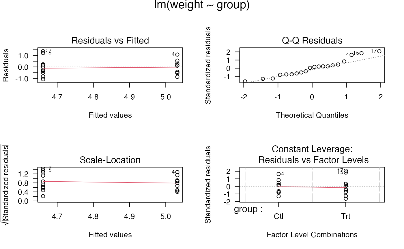

#> 
#> lm> par(opar)
#> 
#> lm> ## Don't show: 
#> lm> ## model frame :
#> lm> stopifnot(identical(lm(weight ~ group, method = "model.frame"),
#> lm+                     model.frame(lm.D9)))
#> 
#> lm> ## End(Don't show)
#> lm> ### less simple examples in "See Also" above
#> lm> 
#> lm> 
#> lm>

Define Your Own Function

Name the function before <-
Define the arguments inside ()
Define what the function does inside {}

pizza <- function(x){ x^2 }
pizza(3)
#> [1] 9

Example Functions

table(penguins$species)
#> 
#>    Adelie Chinstrap    Gentoo 
#>       152        68       124
summary(penguins$bill_length_mm)
#>    Min. 1st Qu.  Median    Mean 3rd Qu.    Max.    NA's 
#>   32.10   39.23   44.45   43.92   48.50   59.60       2

Examples Functions with Missing Data

mean(penguins$bill_length_mm) #returns NA
#> [1] NA
mean(penguins$bill_length_mm, na.rm = TRUE)
#> [1] 43.92193

cor(penguins[ , c("bill_length_mm", "bill_depth_mm", "flipper_length_mm")])
#>                   bill_length_mm bill_depth_mm flipper_length_mm
#> bill_length_mm                 1            NA                NA
#> bill_depth_mm                 NA             1                NA
#> flipper_length_mm             NA            NA                 1
cor(penguins[ , c("bill_length_mm", "bill_depth_mm", "flipper_length_mm")],
    use = "pairwise.complete.obs")
#>                   bill_length_mm bill_depth_mm flipper_length_mm
#> bill_length_mm         1.0000000    -0.2350529         0.6561813
#> bill_depth_mm         -0.2350529     1.0000000        -0.5838512
#> flipper_length_mm      0.6561813    -0.5838512         1.0000000

Other Descriptive Functions

cov()
var()
sd()
scale()

Wrapping Up

In this demo, you’ve learned:
- Some basic programming terminology
- Specific R defaults and issues
- Example functions and use cases
How do I get started?
- Practice!