Hi guys! I have finally done it! I updated my CV with Rmarkdown using Steve’s Markdown Templates. I was tempted to use the new vitae package, but I had already gone down this path before that came out, just finally getting back to it.
Link to the entire CV folder for you to use/view do stuff with: CV. Please ignore the html files in that folder, it does “knit” automatically as part of the website build using markdown - you should be using PDF and LaTex for the CV part.
I decided to do my publications + presentations as an Excel database type file, rather than using a BibTex file. Partially because I dislike BibTex type things, and partially because I like being able to update papers and such as part of a R script (with a little bit of manual control). The slowest part of this process was putting all my current pubs and presentations into the Excel document with my coding system. Let’s look at it:
library(readxl)
curated = as.data.frame(read_excel("../cv/cv_pubs.xlsx"))
names(curated)
## [1] "done" "doi" "title" "osfdoi"
## [5] "author" "journal" "volume" "issue"
## [9] "pages" "year" "pubid" "put-code"
## [13] "pubtype" "pubstatus" "authortype" "category"
## [17] "link" "folder_number"So, I have coded “real” dois (digital object identifiers, like the ones from journals), the title of the paper/prez, the Open Science Framework doi, authors, journal/conference information, volume, issue, pages, and year for citation purposes. Next, I included information from Google Scholar (pubid) and ORCID (put-code). These are useful for updating information, see below. The last was hand coded pubtype (package, article, presentation), pubstatus (published, preprint), authortype (none, under for undergraduate authors, grad for graduate authors, and both), category (psycho and stats), and link for finding the paper or presentation (open science FTW!). I added these categories to be able to format my CV with different groupings based on the current status of a paper, the type of paper (psychological/cognitive science versus statistics), and include a marker of what type of authors there are (hint: loads of students working with me). I use these columns to dynamically create my CV and some of the website pages, since this information updates somewhat frequently. You can view that by looking at the cv markdown, which I can blog about another time.
This post is about how to update your CV with Scholar and ORCID - but using these packages directly gives you a LOT of nonsense (mostly because I don’t spend all data updating the information to be correct on either of these sites, nor do I control what the heck CrossRef/doi.org does when they input the information for dois). Once you have at least one thing entered into an file, you can use this script to update your information, and see what is out there on these two big indexing sites. You would need accounts with Google/ORCID, and I highly recommend both of them to scholars. I have my ORCID to cross reference with CrossRef to add/update entries, and Google Scholar automatically adds all my OSF pre-prints to my site. They also combine references when it’s clear they are the same one (like an OSF page for a project, the journal page for the same paper, etc.).
Start by importing your information from each site:
# pull information from scholar ---------------------------------------------
library(scholar)
erinpubs = get_publications("ReD-s38AAAAJ&hl", #my scholar id
                 cstart = 0, #get everything
                 pagesize = 1000, #max amount of things to get
                 flush = F) #caching parameter
## Warning in get_publications("ReD-s38AAAAJ&hl", cstart = 0, pagesize = 1000, :
## pagesize: 1000 exceeds Google Scholar maximum. Setting to 100.# pull information from orcid ---------------------------------------------
library(rorcid)
erinorc = works(orcid_id("0000-0002-9689-4189"))#my orcid
#note you will have to authorize your orcid for each folder you use this file inEach of these creates a data.frame with different pieces of information - I encourage you to investigate your own. The next thing I did was set up the ORC pages to merge with the Scholar pages. Unfortunately, the ORCID one pulls in a column that’s a list within each cell, so I converted that into a doi (the only variable I wanted) column separately.
# set up dois -------------------------------------------------------------

#blank doi spot
erinorc$doi = NA

#loop over the list to get just the dois
for (i in 1:nrow(erinorc)){

  #grab the list
  temp = erinorc$`external-ids.external-id`[[i]]

  #see if the doi is there
  if (length(temp) > 0 && length(temp[ temp$`external-id-type` == "doi" ,  "external-id-value" ] > 0)) {
    erinorc$doi[i] = temp[ temp$`external-id-type` == "doi" ,  "external-id-value" ]
    } #close if, this handles no dois and multiple ids

  } #close for loop

#take out the duplicates
erinorc = erinorc[!duplicated(erinorc$title.title.value) , ]
Now that we have the two datasets and have extracted the dois, let’s merge them together.
# merge two pub lists -----------------------------------------------------

erinorc$title = erinorc$title.title.value
final = merge(erinpubs, erinorc, by = "title", all = T)
The last piece here is to compare that with my curated list. First, I pulled out all the specific ids that Scholar and ORCID have given my paper. Sometimes, they get multiple ids, so I included them in my curated excel file by doing something like: id1, id2, which makes them easy to split up later.
# compare with curated list -------------------------------------------------
c_pubid = na.omit(unlist(strsplit(gsub(" ", "", curated$pubid), ",")))
c_putcode = na.omit(unlist(strsplit(gsub(" ", "", curated$`put-code`), ",")))
f_pubid = na.omit(unlist(strsplit(gsub(" ", "", as.character(final$pubid)), ",")))
f_putcode = na.omit(unlist(strsplit(gsub(" ", "", final$`put-code`), ",")))
Next, I compared those to the actual ones in Scholar and ORCID:
#find ones that aren't in the curated set from google
google_diff = setdiff(f_pubid, c_pubid)

#find ones that aren't in the curated set from orcid
orc_diff = setdiff(f_putcode, c_putcode)

newrows = final[ final$pubid %in% google_diff |
                   final$`put-code` %in% orc_diff, ]

#create an output for cutting and pasting
curated_check = matrix(NA, nrow = nrow(newrows), ncol = ncol(curated))
colnames(curated_check) = colnames(curated)
curated_check = as.data.frame(curated_check)

curated_check$doi = newrows$doi
curated_check$title = newrows$title
curated_check$author = newrows$author
curated_check$journal = newrows$journal
curated_check$volume = newrows$number
curated_check$year = newrows$year
curated_check$pubid = newrows$pubid
curated_check$`put-code` = newrows$`put-code`

#write.csv(curated_check, "check_these.csv", row.names = F)
setdiff takes the ones that are in the final dataset (f) but aren’t in the curated dataset (c). Then I grabbed the rows in the final dataset that were in the “haven’t seen these yet” pile using %in%. newrows is a list of information found in both of these services that aren’t in your CV. I use the word “new” loosely here. Let’s see what it found, as I’ve just updated my cv.
newrows$title## [1] "Autism Spectrum Disorder and Mitochondrial Dysfunction: The Role of Mitochondrial Dynamics"
## [2] "Clinical practice guideline: Ménière’s disease"
## [3] "Clinical practice guideline: Ménière’s disease executive summary"
## [4] "Code for: Semantic Priming Across Many Languages"
## [5] "Consequences of a telomerase-related fitness defect and chromosome substitution technology in yeast synIX strains"
## [6] "DNA methylation of PGC-1α is associated with elevated mtDNA copy number and altered urinary metabolites in autism spectrum disorder"
## [7] "Dysfibrinogenaemia and caesarean delivery: a case report"
## [8] "Erratum to “A pilot randomized controlled trial testing supplements of omega-3 fatty acids, probiotics, combination or placebo on symptoms of depression, anxiety and stress …"
## [9] "Erratum: Publisher Correction: Situational factors shape moral judgements in the trolley dilemma in Eastern, Southern and Western countries in a culturally diverse sample …"
## [10] "Exploring Metacognition in Statistics Courses"
## [11] "Exploring semantic and executive flexibility interplay in task switching"
## [12] "Increased Mitochondrial Copy Number and Differential DNA Methylation of Mitochondrial Biogenesis and Fusion Genes in a South African ASD Cohort"
## [13] "Many Analysts Project: Gender-inclusive language"
## [14] "Metacognition and Learning During Statistics Courses"
## [15] "Molecular autism research in Africa: a scoping review comparing publication outputs to Brazil, India, the UK, and the USA"
## [16] "Molecular autism research in Africa: emerging themes and prevailing disparities"
## [17] "MSU Group Accelerated CREP--Turri, Buckwalter, Blouw (2015)"
## [18] "Nathan Evans: We have reached a decision regarding your submission to Meta-Psychology,\" What factors are most important in finding the best model of a psychological process …"
## [19] "Peer Review Report"
## [20] "Project IRB Materials"
## [21] "Propionic acid induces alterations in mitochondrial morphology and dynamics in SH-SY5Y cells"
## [22] "Reliability Grades Analysis"
## [23] "Replication of a research claim from Al-Tammemi et al, 2020"
## [24] "Revise 1"
## [25] "Safety and efficacy of non-steroidal anti-inflammatory drugs to reduce ileus after colorectal surgery"
## [26] "Safety of hospital discharge before return of bowel function after elective colorectal surgery"
## [27] "State of Science Paper Guide"
## [28] "Survey_results. Rmd"
## [29] "tag-fig-1. pdf"
## [30] "This is the author's accepted manuscript of an article accepted in Scientific Reports on June 30th, 2025. The final version of record is available online at: https://doi. org …"
## [31] "Timing of nasogastric tube insertion and the risk of postoperative pneumonia: an international, prospective cohort study"
## [32] "Transmission Electron Microscopy Reveals Propionic Acid-induced Alterations to Mitochondrial Morphology in SH-SY5Y Cells"
## [33] "Updated Registration-Big Team Science"
## [34] "Validation of the OAKS prognostic model for acute kidney injury after gastrointestinal surgery"
## [35] "word-fig-1. png"These three are 1) OSF page for an Accelerated CREP I am on, but I haven’t added it yet to my CV because it’s a bit early to be sharing (i.e., waiting until there’s more of real paper there), 2) a “preprint” project we did for one of my classes, and 3) I have no idea, since that doi is linked to APA’s website, which I don’t have access to. Probably a doi for a conference presentation, but I don’t really know or care much. I could exclude these from future searches by adding a line to my curated excel sheet that includes these pubids and put-codes. Because I use the pubtype columns to print things out on my CV, they would get ignored as things not to print.
This next part is set up to help me figure out when articles actually go to press to update their volume information, but you could change the next bit of code to find any differences in your information you might be interested in. Scholar does give you citation rates, but that’s not really my thing to track (however, for some folks working at institutions that do care, you could update that over time using something like this code).
#update any X or XX that were place holders for the pages
temp = na.omit(curated[ , c("pubid", "volume")])
update = temp$pubid[temp$volume == "X"]

final[final$pubid %in% update, c("title", "number")]
## title
## 82 Differential Effects of Association and Semantics on Priming and Memory Judgments.
## 95 Evaluating interventions: A practical primer for specifying the smallest effect size of interest
## 141 Investigating object orientation effects across 18 languages
## 237 Semantic Feature Production Norms
## 267 The reliability of student evaluations of teaching
## number
## 82
## 95 127-135
## 141
## 237
## 267 1-15None of these have new volume or page numbers, so I am good to go here. Because I have this as an excel sheet, I can do some fun visualizations:
library(ggplot2)

ggplot(curated[ curated$pubtype == "article" & curated$pubstatus == "published", ],
       aes(as.numeric(year))) +
  geom_histogram(stat = "count", bins = 1) +
  theme_bw() +
  geom_vline(xintercept = 2008) +
  geom_vline(xintercept = 2010, color = "blue") +
  geom_vline(xintercept = 2014, color = "maroon") +
  geom_vline(xintercept = 2018, color = "green") +
  ylab("Pub Count") +
  xlab("Year")
## Warning in geom_histogram(stat = "count", bins = 1): Ignoring unknown
## parameters: `binwidth`, `bins`, and `pad`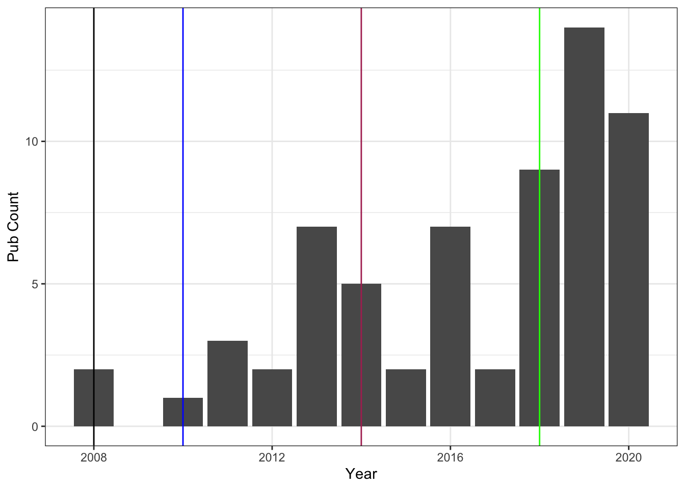
Publication rates over years don’t always make sense to me because often the year something is “published” is one to two years after it was finally accepted - and let’s not even talk about how long that can take sometimes to get from just submitted to accepted. But it’s fun to look at sometimes … major career events are marked on the graph:
- Black: finished Ph.D., got a teaching type position
- Blue: moved to a tenure track position
- Maroon: Assistant to Associate Professor, tenured
- Green: changed jobs and was hired as a full Professor
Graduate school was not the smoothest adventure for me, which is a story best left for in person communication … and you can see that it affected my ability to publish in my early years (if we want to consider ourselves the whole of our output rates, which I think is dumb). The other interesting part about this graph is the middle period between my tenure and now … that’s another story best left for in person communication. Sometimes life makes science difficult and these were definitely difficult years job-wise.
A more important graph for me (if we focus solely again on publications) is this:
curated$authortype = factor(curated$authortype,
                            levels = c("none", "under", "grad", "both"),
                            labels = c("Just PhDs", "Undergraduates", "Graduates", "Both"))

ggplot(curated[ curated$pubtype == "article" & curated$pubstatus == "published", ],
       aes(authortype)) +
  geom_histogram(stat = "count", bins = 1) +
  theme_bw() +
  ylab("Pub Count") +
  xlab("Authorship Type")
## Warning in geom_histogram(stat = "count", bins = 1): Ignoring unknown
## parameters: `binwidth`, `bins`, and `pad`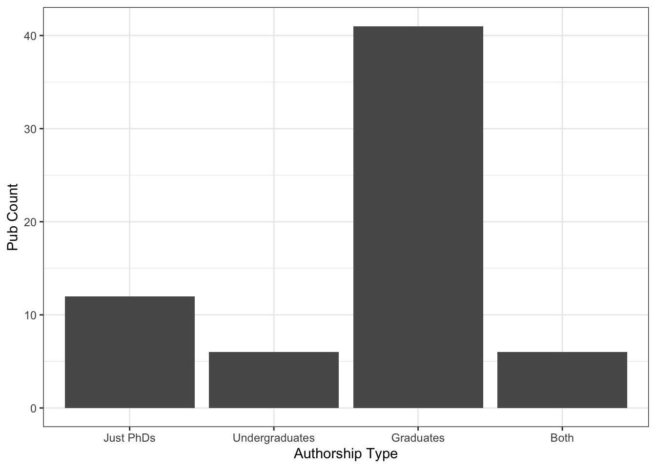
Students are a priority! Thank you for coming to my TED talk. I don’t even know that I could graph the conference presentations in a good way, but it follows the same trend. And that’s a much better statistic to be proud of than counts per year.
Hope you can use these code bits to help with your bean counting - questions welcome and more on the markdown template later.